GSEA User Guide

Introduction#

Gene Set Enrichment Analysis (GSEA) is a computational method that determines whether an a priori defined set of genes shows statistically significant, concordant differences between two biological states (e.g. phenotypes). The Gene Set Enrichment Analysis PNAS paper fully describes the algorithm. The GSEA software makes it easy to run the analysis and review the results, allowing you to focus on interpreting the analysis results.

The basic steps for running an analysis in GSEA are as follows:

1. Prepare your data files. See Preparing Data Files for GSEA.

• Expression dataset file (res, gct, pcl, or txt)
• Phenotype labels file (cls)
• Gene sets file (gmx or gmt)
• Chip (array) annotation file (chip)

2. Load your data files into GSEA. See Loading Data.
3. Set the analysis parameters and run the analysis. See Running Analyses.
4. View the analysis results. See Viewing Analysis Results.

Installing and Starting GSEA#

To start GSEA, select and download the appropriate GSEA package for your operating system from the Downloads page of the GSEA website.

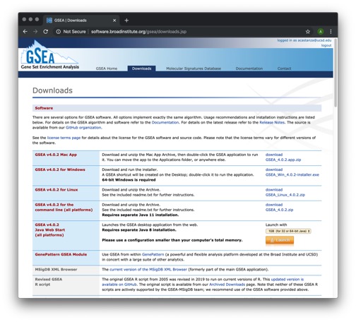
You can run GSEA in multiple ways:

• The GSEA desktop application provides an easy-to-use graphical interface. The Downloads page provides GSEA application bundles for Linux, Mac, and Windows, each providing an embedded platform-specific version of Java, making it unnecessary to install Java separately. Further instructions are available on the website. The GSEA desktop application can also be launched directly from the Downloads page using Java Web Start technology (http://java.sun.com/products/javawebstart/) to download, install, and start the application.
• GSEA analyses can be run on the command line as described in Running GSEA from the Command Line. You can download a .zip file with this version of GSEA from the Downloads page. The Linux bundle for the desktop application also provides the option to run from the command line.
• R-GSEA makes GSEA available from the R programming environment. Links to this version are provided on the Downloads page.
• There are cloud-accessible modules available through GenePattern for GSEA and GSEAPreranked analyses equivalent to those in the GSEA desktop application. There is also a module for the related ssGSEAProjection analysis (discussion of this is beyond the scope of this guide; please see the GenePattern site for more information).

This guide focuses on the GSEA desktop application and provides instructions for running GSEA from the command line. It does not provide information about R-GSEA or the GenePattern modules.

When you start the GSEA desktop application, the main window appears with the Home page displayed:

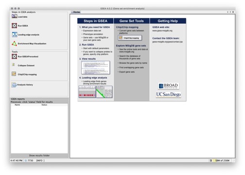
The icons on the left provide quick access to the most common actions. Typically, each action you select opens a new page in the GSEA window. For example, selecting the Load Data icon opens the Load Data page.

The Processes pane in the bottom left corner of the GSEA window displays status information when you run an analysis.

GSEA user preferences are stored in the gsea_home directory (Help>Show GSEA home folder). GSEA analysis reports are stored in the GSEA output folder (Help>Show GSEA output folder). To change the location of the GSEA output folder and other preferences, use the Preferences Window.

The GSEA desktop application can be run without being connected to the internet. You can use most functions in GSEA without an internet connection; for example, you can load files, run analyses, and review analysis results. However, you need to be connected to the internet to view the GSEA documentation (including online Help), access the GSEA website, or access the hosted files (MSigDB gene sets and array annotations) on the GSEA-MSigDB file servers.

Getting Help#

The GSEA website is your primary source of help for GSEA. It includes the following resources:

• Documentation. The GSEA documentation includes this User Guide, a Tutorial that walks you through key features of GSEA, and a FAQ that answers frequently asked questions.
• MSigDB, the Molecular Signature Database. This database provides curated gene sets for use with the gene set enrichment analysis. Each gene set is described by a gene set page.
• Publications. The website provides a link to the Gene Set Enrichment Analysis PNAS paper.
• Array annotation files. Each file lists the identifiers used by a gene expression quantification technology and their matching HGNC gene symbol. GSEA uses these “chip” annotation files to translate between platform specific gene identifiers and approved gene symbols, and to include gene annotations in the gene set enrichment analysis report.
• Example datasets. The datasets used in the Gene Set Enrichment Analysis PNAS paper and other publications.

If you cannot find the answers to your questions in the manual or the FAQ, please contact us.

---

Preparing Data Files for GSEA#

When you use GSEA, you supply four data files: an expression dataset file, phenotype labels file, gene sets file, and chip annotations file. The following table lists each data file and its valid file formats. All files are tab-delimited ASCII text files; they can be created and edited using any text editor.

For descriptions and examples of each file format, see GSEA file formats. For more information about each data file, click the data file link in the following table:

Data File	Content	Format	Source
Expression dataset	Contains features (genes or probes), samples, and an expression value for each feature in each sample. Expression data can come from any source (Affymetrix, Stanford cDNA, and so on).	res, gct, pcl, or txt	You create the file.
Phenotype labels	Contains phenotype labels and associates each sample with a phenotype.	cls	You create the file or have GSEA create it for you.
Gene sets	Contains one or more gene sets. For each gene set, gives the gene set name and list of features (genes or probes) in that gene set.	gmx, gmt or grp	You use the files hosted on the GSEA-MSigDB file servers, export gene sets from the Molecular Signature Database (MSigDB), or create your own gene sets file.
Chip annotations	Lists each identifier on a platform and its matching HGNC gene symbol. Optional for the gene set enrichment analysis.	chip	You use the files hosted on the GSEA-MSigDB file servers, download the files from the GSEA website, or create your own chip file.

Consistent Feature Identifiers Across Data Files#

The expression dataset, gene sets, and chip annotation files all contain lists of features (genes or probes) to be analyzed. It is critical that you use the same feature (gene or probe) identifiers across all of the data files.

Typically, the feature identifiers in your expression dataset are the identifiers for the assay used to produce the data, either microarray probe identifiers or transcriptomic gene identifiers. For example, an expression dataset produced using the HG_U133A chip contains HG_U133A probe identifiers and an expression dataset produced using the HG_U95Av2 chip contains HG_U95Av2 probe identifiers. When using GSEA, it is critical that your expression dataset, gene sets, and chip annotation files all use compatible feature identifiers.

Typically, you use one of two approaches to ensure that you are using consistent feature identifiers across files: you collapse your probe sets into genes and use the HGNC gene symbols as your consistent feature identifiers or you use the identifiers from your expression dataset as your consistent feature identifiers.

• HGNC gene symbols. To use HGNC gene symbols as your consistent feature identifiers:

  • Specify your expression dataset.
  • Set the Collapse/Remap to gene symbols parameter when you run the gene set enrichment analysis:
    • Set the parameter to “Collapse” to indicate that you want to use gene symbols. This causes GSEA to collapse the probe sets in the dataset to a single vector for the gene, which gets identified by its HGNC gene symbol. Collapsing the dataset has two benefits: (1) it eliminates multiple probes, which can inflate enrichment scores, and (2) it facilitates the biological interpretation of the gene set enrichment analysis results. This parameter requires you to specify an accompanying chip file.
    • Alternatively, your dataset may already contain unique gene symbols. If they are from an older genome than the current target MSigDB version, then set the parameter to “Remap_Only” and specify an appropriate chip file to perform the symbol remapping. Or set the parameter to “No_Collapse” if your dataset contains gene symbols that already match the current MSigDB version (you may find that a sufficiently recent genome sufficient as well).
  • Specify gene sets that list genes by their HGNC gene symbol. The gene sets on the GSEA-MSigDB file servers are from the Molecular Signature Database (MSigDB) and list genes by HGNC gene symbol.
  • Specify a chip annotation file that maps the probe identifiers in your expression dataset to their HGNC gene symbols. GSEA uses the chip annotation file to collapse each probe set into a single vector for the gene, which gets identified by its HGNC gene symbol, and to include HGNC gene annotations in the analysis report.

  This approach is recommended by the GSEA team; therefore, by default the Collapse/Remap to gene symbols parameter is set to “Collapse”.

• Non-Symbol identifiers. To use non-symbol identifiers, such as microarray probe identifiers, or other gene ids as your consistent feature identifiers:

  • Specify your expression dataset.
  • Set the Collapse/Remap to gene symbols parameter to “No_Collapse” when you run the gene set enrichment analysis. This indicates that you want to use the native identifiers in your dataset and GSEA does not collapse the identifiers in your expression dataset. You are choosing to analyze the identifiers directly rather than in the namespace of approved HGNC gene symbols.
  • Specify gene sets that list genes using the same identifiers as those in your expression dataset (that is, the same identifiers for the pipeline used to produce your expression dataset). You cannot use the gene sets on the GSEA-MSigDB file servers because they list genes by HGNC gene symbol. However, you can export gene sets from the MSigDB, specifying the chip used to produce your expression dataset as the target chip for the exported gene sets file.

  This approach is useful if you prefer not to use the HGNC gene symbols or your expression dataset contains identifiers that cannot be mapped to the HGNC gene symbols. For example, if you have an expression dataset produced using porcine DNA, you cannot map the porcine identifiers to HGNC gene symbols, which means you cannot create a chip annotation file. However, you can create gene sets that contain porcine probe identifiers, which means you can still run the gene set expression analysis.

One final note concerning consistent feature identifiers across files: within GSEA, HGNC gene symbols and probe identifiers are case sensitive; that is, the identifiers “TestGene1” and “TESTGENE1” are not the same.

Expression Datasets#

An expression dataset file contains features (genes or probes), samples, and an expression value for each feature in each sample. It is a tab-delimited text file in gct, res, pcl, or txt format. For descriptions and examples of each file format, see GSEA file formats.

Because most gene expression data is already in tab-delimited text files, or in spreadsheet and database programs that allow you to export the data into tab-delimited text files, creating expression dataset files for GSEA is relatively easy:

1. Start with a tab-delimited file that contains your gene expression data.
2. Open the file in Excel or a text editor.
3. Make the necessary format changes: compare your current file with the file format described in GSEA file formats; add header rows, remove extra columns, and make any other changes necessary to create a properly formatted file.
4. Save the file as a tab-delimited text file with the appropriate file extension (gct, res, pcl, or txt). Note: GSEA expects a very specific formatting for .txt files. See the file formats page for details. Also, be aware that some editors on some platforms automatically attach the “txt” extension to other file types (e.g. “.gct.txt”), which may confuse GSEA during parsing. Make sure to remove the extra .txt extension from the name before using the file with GSEA.

Note: When you create an expression dataset file, the GSEA team recommends that the file name include the name of the chip used to produce the expression data; for example, all_aml_dataset_hgu95av2.gct.

When creating expression dataset files, keep in mind the following:

• Expression data. GSEA works with expression data from any source. Although different processing methods produce different types of expression values (for example, natural scale versus logged expression levels for Affymetrix data, or Affymetrix data versus two-color ratio data), any type of expression values can be used to create your expression dataset file. The GSEA algorithm examines the differences in expression values, rather than the values themselves. (As in most data analysis methodologies, the same expression data represented in different formats may, of course, generate different analysis results.)
• Image data. GSEA does not process image data. If you have image data, you must use external software (such as Rosetta Resolver or Stanford Microarray Database) to convert the image data to numeric data.
• RNA-seq data. GSEA does not normalize RNA-seq data. RNA-seq data must be normalized for between-sample comparisons using an external normalization procedure (e.g. those in DESeq2 or Voom).
• cDNA two-color ratio data. See cDNA Microarray Data.
• CEL files. If you are analyzing CEL files, each of which contains data for one sample, you will need to merge the collection of CEL files into a single expression dataset file. You can use the GenePattern module ExpressionFileCreator to merge CEL files into an expression dataset file. Alternatively, you can use tools such as RMAExpress or DCHIP to merge the CEL files and then create your expression dataset file based on that merged file.
• Genes. Each feature (gene or probe) must have a unique identifier. If the expression dataset contains redundant identifiers, GSEA arbitrarily selects one of the redundant features, removes the others and continues the analysis. The analysis report lists the redundant identifiers.
• Samples. Each sample must have a unique identifier. If you have technical replicates, you generally want to remove them by averaging or some other data reduction technique. For example, assume you have five tumor samples and five control samples each run three times (three replicate columns) for a total of 30 data columns. You would average the three replicate columns for each sample and create a dataset containing 10 data columns (five tumor and five control).
• Present/Marginal/Absent Calls. GSEA ignores Present/Marginal/Absent calls. If your dataset contains such calls, do not filter the data based on that information. The GSEA algorithm expects different levels of expression and provides better results when given all of the data.

• Missing expression values. The gct, txt, and pcl file formats support missing expression values; simply leave the cell blank if the expression data is missing. The res file format, which is specific to Affymetrix chips, does not allow missing expression values. You can run the gene set enrichment analysis against an expression dataset that is missing values. The GSEA software does not impute missing values or filter out genes that have too many missing values; it simply ignores the missing values in its ranking metric calculations. However, too many missing values for a gene may cause the differential expression scores for that gene to be inaccurate. For example, consider a dataset that contains 10 samples in class_A and 15 samples in class_B. Assume that a gene has only 3 values in class_A and all 15 values in class_B. The GSEA software uses the 3 values in class_A and the 15 values in class_B to score the gene by its differential expression. In the signal-to-noise calculation, the mean and variance estimates for the gene are based on different sample sizes; a situation which it would be better to avoid. (If you wish, you can use external tools to impute missing values or filter out genes that have too many missing values.)

• Filtering based on expression values. For many other analytical algorithms, such as clustering, it makes sense to pre-process a dataset. For example, before running hierarchical clustering, you might remove genes that have low variance across the dataset. This prevents flat genes from driving the clustering result and improves processing time by focusing on a smaller number of interesting genes. The GSEA algorithm does not filter the expression dataset and generally does not benefit from your filtering of the expression dataset. During the analysis, genes that are poorly expressed or that have low variance across the dataset populate the middle of the ranked gene list and the use of a weighted statistic ensures that they do not contribute to a positive enrichment score. By removing such genes from your dataset, you may actually reduce the power of the statistic and processing time is rarely a factor as GSEA can easily analyze 22,000 genes with even modest processing power. However, an exception exists for RNA-seq datasets where GSEA may benefit from the removal of extremely low count genes (i.e., genes with artifactual levels of expression such that they are likely not actually expressed in any of the samples in the dataset). Although GSEA does not require that you preprocess the expression dataset, it can be used effectively on preprocessed datasets. For example, Monti et al used a filtered dataset to further analyze genes consistently expressed across two datasets, as described in “Molecular profiling of diffuse large B-cell lymphoma identifies robust subtypes including one characterized by host inflammatory response” (http://www.bloodjournal.org/cgi/content/full/bloodjournal;105/5/1851).

Phenotype Labels#

A phenotype label file, also known as a class file or template file, defines phenotype labels and assigns those labels to the samples in your expression dataset. A phenotype label file is a tab-delimited text file in cls format. For descriptions and examples of the cls file format, see GSEA file formats.

• About Phenotype Labels
• Creating Phenotype Labels
• Selecting Phenotypes Labels to Analyze

About Phenotype Labels#

The GSEA algorithm works with both categorical labels and continuous labels:

• A categorical label defines a discrete phenotype. If you are using categorical labels, you must define at least two labels (for example, tumor and normal), but you may define as many as necessary (for example, ALL, MLL, and AML). The GSEA algorithm analyzes two labels at time (for example, ALL versus MLL or ALL versus not_ALL). If you choose to analyze two labels and your phenotype file contains more than those two labels, GSEA analyzes only the samples with the selected labels and omits all other samples from the analysis. This makes it easy to analyze subsets of your expression datasets.

• A continuous label defines a phenotype profile, which is used to analyze a time series experiment or to find gene sets that correlate with a gene of interest (gene neighbors). A continuous label contains a value for each sample, where that series of values defines the phenotype profile:

  • For a gene of interest, the value for each sample is the expression value of the gene. The phenotype profile is, therefore, the expression profile of the gene of interest.

  • For a time series, the value for each sample is a number chosen to define the desired expression profile. The relative change in the value for each sample defines the relative distance between points in the profile. Assume, for example, that you have five samples taken at 30 minute intervals. To define a phenotype profile that shows steadily increasing gene expression, you would choose steadily increasing values for each sample (perhaps the number of minutes elapsed since the initial treatment):

  #numeric
  #IncreasingProfle
  30 60 90 120 150

  To define a phenotype profile that shows an initial peak and then gradual decrease, you would choose values for each sample that reflect that desired phenotype profile:

  #numeric
  #PeakProfle
  5 20 15 10 5

Creating Phenotype Labels#

To create a phenotype labels file:

1. Open Excel or a text editor.
2. Create the phenotype label file using the cls file format (see GSEA file formats). Every label defined in the phenotype labels file must be assigned to at least one sample in the expression dataset. Every sample in the expression dataset must be assigned a label. The order of the labels in the cls file is important; see GSEA file formats for details. Save the file as a tab-delimited text file with the file extension cls.

Typically, you create a phenotype label file before running the gene set enrichment analysis; however, you can also have GSEA create phenotype label files for you when you run the analysis, as described in the next section.

Selecting Phenotype Labels to Analyze#

When you run the gene set enrichment analysis, you select a continuous phenotype label or a pair of categorical phenotype labels. When you run an analysis using the Run GSEA Page, you can select the phenotype labels in the following ways:

• Select a phenotype labels file that you have created and select a continuous phenotype label or a pair of categorical phenotype labels from that file.
• Create an on-the-fly phenotype. GSEA presents a dialog box that allows you to define two categorical phenotype labels. You enter the name of the dataset that you are using, two phenotype labels, and the samples from your dataset that are associated with each phenotype. GSEA ensures that the samples are in your dataset and creates the phenotype labels file for you. If your dataset contains samples that you did not include in the two phenotypes, GSEA automatically excludes them from the gene set enrichment analysis.
• Use a gene as a phenotype. You select a gene from your dataset and GSEA creates a continuous phenotype label file for you. In the phenotype file, the value for each sample is the expression value of the gene that you selected.

Gene Sets#

A gene sets file defines one or more gene sets. For each gene set, the file contains the gene set name and the list of genes in that gene set. A gene sets file is a tab-delimited text file in gmx or gmt format. For descriptions and examples of each file format, see GSEA file formats.

The Molecular Signature Database (MSigDB) is a publicly accessible collection of curated gene sets that is maintained by the GSEA team. The team appreciates contributions to this shared resource and encourages users to submit their gene sets to genesets@broadinstitute.org.

• Selecting Hosted MSigDB Gene Sets
• Exporting Gene Sets from MSigDB
• Creating Gene Sets
• Gene Sets and GSEA

Selecting Hosted MSigDB Gene Sets#

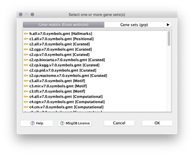
When you run an analysis, you can select from a menu of MSigDB gene set files hosted by the GSEA team. The file name indicates the content of the file. For example, the gene set file c2.all.v7.0.symbols.gmt, contains all C2 gene sets from version 7.0 of the MSigDB with the genes in the gene sets identified by HGNC gene symbol.

For a list of the gene set files on the website, click the Run GSEA icon to display the Run GSEA page and click the … button next to the Gene sets database parameter:

Exporting Gene Sets from MSigDB#

You can use the MSigDB XML Browser application to explore the gene sets in the MSigDB and to export gene sets of interest to gene set files. To display the gene sets, click the Load database button:

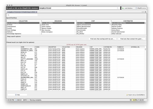
From this page, you can:

• Use the fields at the top of the page to filter the gene sets displayed in the table.
• Select a gene set from the table and right-click to display information about the gene set.
• Export selected gene sets to a gene set file, selecting the feature identifiers (gene symbols or DNA chip platform of your choice) that you want to use to identify the genes in the gene sets.

For more information, see the MSigDB XML Browser section of this Guide. Alternatively, you can use the online tools on the MSigDB website to export gene sets.

Creating Gene Sets#

To create your own gene sets file:

1. Open Excel or a text editor.
2. Enter the gene sets details using the gmx or gmt file format (see GSEA file formats). When listing the genes in each gene set, be sure to use the appropriate gene identifiers (HGNC gene symbols or probe identifiers), as described in Consistent Feature Identifiers Across Data Files.
3. Save the file as a tab-delimited text file with the appropriate file extension (gmx or gmt).

Note: When you create a gene sets file, the GSEA team recommends that the file name include the gene identifier format you used to list the genes; for example, setname_hgu95av2.gct. Also, be aware that some editors on some platforms automatically attach the “txt” extension to other file types (e.g. “.gmt.txt”), which may confuse GSEA during parsing. Make sure to remove the extra .txt extension from the name before using the file with GSEA.

Gene Sets and GSEA#

When choosing gene sets for a gene set enrichment analysis, keep in mind the following:

• When you run the gene set enrichment analysis, the GSEA software automatically preprocesses the gene sets, and excludes any gene that is not in the expression dataset. For example, if you restricted a 22,000 gene HGU133A dataset to the 5,000 most reproducible genes, the GSEA software first discards all genes in the gene sets that are not in the restricted dataset and then continues with the analysis. Preprocessing the gene sets is critical because the gene set size affects the enrichment score statistic. It is not recommended to manually rescript the input expression data set in most cases. As noted in Expression Datasets above, the GSEA software does not preprocess the expression dataset. The expression dataset may contain a significant number of genes that are not in any of the gene sets. The GSEA algorithm simply asks if the genes in a gene set are overrepresented at the top or bottom of the ranked list of genes from the expression dataset.
• When you run the gene set enrichment analysis, the GSEA software automatically normalizes the enrichment scores for variation in gene set size, as described in GSEA Statistics. Nevertheless, the normalization is not very accurate for extremely small or extremely large gene sets. For example, for gene sets with fewer than 10 genes, just 2 or 3 genes can generate significant results. Therefore, by default, GSEA ignores gene sets that contain fewer than 15 genes or more than 500 genes; defaults that are appropriate for datasets with 10,000 to 20,000 features. To change these default values, use the Max Size and Min Size parameters on the Run GSEA Page; however, keep in mind the possibility of inflated scorings for very small gene sets and inaccurate normalization for large ones.
• GSEA analysis results include a report that lists the gene sets included in and excluded from the analysis. For each gene set included in the analysis, the report lists the total number of genes in the set and the number of genes in the set after filtering out genes that are not in the expression dataset.
• When you run the gene set enrichment analysis, try to avoid the occurrence of highly similar gene sets within the gene set database. Because the false discovery rate (FDR) statistic is based on all gene sets, duplicate or near duplicate gene sets can skew this critical statistic.

Chip Annotations#

A chip annotations file lists each identifier used in a platform and its matching HGNC gene symbol. A chip annotations file is a tab-delimited text file in chip or csv format. For descriptions and examples of the chip annotations file formats, see GSEA file formats.

• How GSEA Uses Chip Annotations
• Selecting Hosted Chip Annotations
• Creating Chip Annotations

How GSEA Uses Chip Annotations#

When you run the gene set enrichment analysis (Run GSEA or GSEAPreranked):

• GSEA uses the selected chip annotation files to include HGNC gene annotations in the analysis report. If you do not select a chip annotation file, the analysis report displays the gene descriptions from the expression dataset file. If you select a chip annotation file, GSEA includes HGNC gene annotations in the analysis report.
• If you are collapsing your dataset (i.e., you set the Collapse/Remap to gene symbols parameter to “Collapse” or “Remap_Only”), GSEA uses the selected chip annotation files to map each identifier in the expression dataset file into a single vector for the gene, which is identified by its HGNC gene symbol.

Also, when you use Chip2Chip to translate a gene set from gene symbols to the identifiers of a chip platform, the selected chip annotation file is used to translate HGNC gene symbols in the gene sets to the matching probe identifiers for the target chip(s). This can be thought of as reading the chip file backwards.

When you use the MSigDB XML Browser to export gene sets from the MSigDB, you select a target chip for the gene sets. Chip2Chip and the selected chip annotation files are used to translate the HGNC gene symbols in the MSigDB gene sets to the matching probe identifiers for the target chip.

Selecting Hosted Chip Annotations#

When you run an analysis, you can select from a menu of chip annotation files hosted on the GSEA-MSigDB file servers. These files are created and maintained by the GSEA team for your convenience. They include chip annotation files for commonly used platforms present in the Ensembl Biomart (human, mouse, and rat), as well as three specially defined chip files:

• Human_Symbol_with_Remapping_MSigDB.vX.chip
• Mouse_Symbol_with_Remapping_MSigDB.vX.chip
• Rat_Symbol_with_Remapping_MSigDB.vX.chip

These special chip files are designed to provide “roll-up” updates for gene symbols used in older versions of genome annotations for their respective species to the versions of HGNC gene symbols used in the specific version of MSigDB targeted by the file.

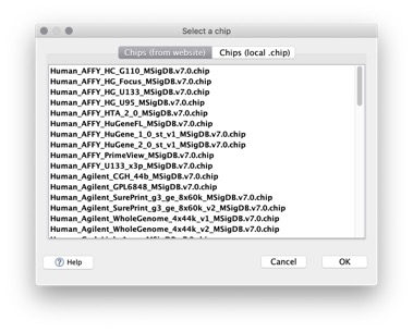
For a list of the hosted chip annotation files, click the Run GSEA icon to display the Run GSEA page and click the … button next to the Chip platform(s) parameter.

Creating Chip Annotations#

If you cannot find a chip annotations file for the chip that you are using, you can create one. Creating a chip annotations file is easy; however, mapping your probe identifiers to HGNC gene symbols may be difficult or impossible. To create a chip annotations file:

1. Start with a tab-delimited file (or text file) that lists the probes on the chip. The chip manufacturer generally provides this file.
2. Open the file in Excel or a text editor. If using Excel be sure to import the data as “text” formatted columns and not “general”.
3. Make the necessary format changes: compare your current file with the chip file format described in GSEA file formats; add header rows, remove extra columns, and make any other changes necessary to create a properly formatted file.
4. Using the information you have available (for example, ortholog data), determine the matching HGNC gene symbol for each probe and add it to the file. If you cannot determine the HGNC gene symbol it can be left out of the file entirely as it will not map to any gene set member in that case. Alternatively, if you wish to keep the probe as a placeholder or for informational purposes, you can add it to the file but leave the gene symbol blank so it won’t map to anything. As mentioned above, depending on the chip that you are using, it may be difficult or impossible to determine matching gene symbols.
5. Save the file as a tab-delimited text file with the file extension .chip.

Note: (1) The file name must not include hyphens (-). (2) When you create a chip annotation file, the GSEA team recommends that the file name be the name of DNA chip; for example, hgu95av2.chip. Also, be aware that some editors on some platforms automatically attach the “txt” extension to other file types (e.g. “.chip.txt”), which may confuse GSEA during parsing. Make sure to remove the extra .txt extension from the name before using the file with GSEA.

cDNA Microarray Data#

An expression dataset file for cDNA ratio data contains features (genes or probes), samples, and a computed ratio value for each feature in each sample. A phenotype label file for cDNA ratio data assigns distinct phenotype labels to the samples in the expression dataset.

Ratio values for cDNA data can be computed using a variety of methods. How the ratios are computed determines whether it is possible to create a phenotype label file for the cDNA ratio data. For example:

• If ratios for all samples are computed against a common reference, as shown below, each sample can be assigned a distinct phenotype and it is possible to create a phenotype label file.

  normal sample (Cy3) / common reference (Cy5) = phenotype 1
  treated sample (Cy3) / common reference (Cy5) = phenotype 2

• If ratios are computed by comparing conditions, as shown below, it may not be possible to create a phenotype label file.

normal sample (Cy3) / treated sample (Cy5) = phenotype

When you run the gene set enrichment analysis from the Run GSEA Page, GSEA ranks the features in the expression dataset and then analyzes the ranked list of features. GSEA provides a number of metrics for ranking genes; however, all of the metrics require a phenotype label file. Alternatively, you can create a ranked list of the features in the expression dataset and then use the GSEAPreranked Page to analyze that ranked list.

If you can assign distinct phenotypes to the samples in the cDNA ratio data, analyze the data using the Run GSEA page:

1. Create an expression dataset file for the cDNA ratio data. The file must be formatted as a pcl, res, gct, or txt file. For descriptions and examples of these file formats, see GSEA file formats. Note: If the raw expression data contains two separate values for each gene in each sample, use external software to calculate the two-color ratios before creating the expression dataset file.
2. Create a phenotype label file that assigns a distinct phenotype label to each sample in the expression dataset file. The file must be formatted as a cls file. For a description of this file format, see GSEA file formats.
3. Run the analysis using the Run GSEA Page.

If you cannot assign distinct phenotypes to the samples in the cDNA ratio data, analyze the data using the GSEAPreranked page:

1. Rank the features in the expression dataset using tools external to GSEA.
2. Create a ranked list file that contains the rank ordered list of features. The file must be formatted as an rnk file. For a description of this file format, see GSEA file formats.
3. Run the analysis using the GSEAPreranked Page.

When selecting the chip platform(s) to use for analyzing cDNA data, the GSEA team recommends selecting both the Stanford and seq_accession chip annotation files. This helps to ensure that any non-standard cDNA identifiers in your dataset are used in annotating the analysis reports and/or collapsing the dataset (see Consistent Feature Identifiers Across Data Files).

---

Loading Data#

Before you can run an analysis, you must load the expression dataset (res, gct, pcl, or txt), phenotype label (cls), and gene set files (gmx or gmt) to be analyzed. Loading the files stores the data in memory, where GSEA can work with them. You must load the data files into GSEA each time you open the application.

To load the data files, click the Load Data icon in the Navigator area of the GSEA window. GSEA displays the Load Data page:

From the Load Data page, you can load files in four ways:

• Click the Browse for files button. When the Open window appears, select the file(s) to load and then click the Open button. To select multiple files, use SHIFT-click or CTRL-click.
• Click the Load last dataset used button. GSEA loads the data used in the most recent gene set enrichment analysis.
• Drag-and-drop the files from a file browser window into the drag-and-drop pane. When the files that you want to load are listed in that pane, click the Load these files button. To remove files from the drag-and-drop pane, click the Clear button.
• In the Recently Used Files pane, double-click a file to load it.

GSEA loads the files and adds them to the Recently Used Files and Object Cache panes (if they are not yet listed):

• Recently Used Files lists the files that you have loaded into GSEA during this session and previous sessions. Files remain in this pane, even when you exit and restart GSEA, unless you select File>Clear Recent File History to clear them.
• Object Cache lists the files you have loaded during this session. When you restart GSEA, the Object Cache is empty.

The icon next to a file name identifies the type of data it contains.

Select a file in the Recently Used Files or Object Cache pane and right-click in that area to display a context menu of tools appropriate for the selected file(s):

Tool	Description	Notes
Dataset Viewer	Opens a page in the GSEA window that displays the expression dataset.	Expression datasets only
Phenotype Viewer	Opens a page in the GSEA window that displays the phenotype labels and the number of samples associated with each.	Phenotype labels only
Report Viewer	Opens a page in the GSEA window that displays the analysis report, as it appears in the Analysis History page.	Reports only
Gene Matrix Viewer	Opens a page in the GSEA window that displays the gene set data.	Gene sets (database) only
Extract GeneSets from GeneMatrix	Creates a gene set group (grp) for each gene set in the gene set file. The gene sets are created in memory and deleted when you exit from GSEA. When you run an analysis and need to select gene sets for the analysis, you will see the new gene sets listed in the gene set selection window.	Gene sets (database) only
Convert the GeneMatrix into a Single GeneSet	Creates one gene set group (grp) that combines the genes in all of the gene sets into one large gene set. The gene set is created in memory and deleted when you exit from GSEA. When you run an analysis and need to select gene sets for the analysis, you will see the new gene set listed in the gene set selection window.	Gene set (database) only
Gene Set Viewer	Opens a page in the GSEA window that displays the genes in the gene set.	Gene sets (group) only
Remove duplicates from the GeneSet	Removes duplicate genes from the gene set, overwriting the original gene set with the new gene set.	Gene sets (group) only
View Chip Annotation	Opens a page in the GSEA window that displays the probe to symbol mapping in the chip annotation file. (Typically, you do not load chip annotation files.)	Chip annotations only
Ranked List Viewer	Opens a page in the GSEA window that displays the ranked list of genes. For a ranked list file generated by GSEA, the display includes rank and rank metric scores.	Ranked lists only
Force Data Reload.	Loads the selected file again, overwriting the previously loaded data.	All files
Copy Files	Copies the full path of the selected files to the clipboard. You can then paste that file name where needed.	All files, Recently Used Files only
Import Data	Loads the selected files.	All files, Recently Used Files only

---

Running Analyses#

The primary analysis that you run in GSEA is the gene set enrichment analysis; however, GSEA also offers other tools, which are run as analyses. This section describes how to start and track analyses:

• Running a Gene Set Enrichment Analysis
• Running a Leading Edge Analysis
• Running Other GSEA Analyses
• Tracking Analysis Progress
• Rerunning an Analysis

Running a Gene Set Enrichment Analysis#

As described in the Gene Set Enrichment Analysis PNAS paper, the gene set enrichment analysis is a computational method that determines whether an a priori defined set of genes shows statistically significant, concordant differences between two biological states (e.g. phenotypes).

To start a gene set enrichment analysis:

1. Select the Run GSEA icon on the GSEA main page. The GSEA page appears:

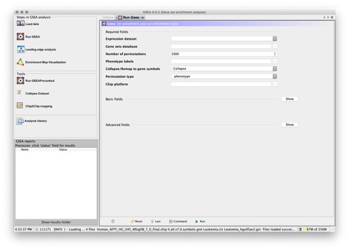
2. Enter values for the parameters listed under Required Fields. Optionally, click Show to display the parameters under Basic Fields and Advanced Fields and enter values for those parameters as well. For descriptions of the parameters, click Help, which displays the Run GSEA Page of this guide.
3. Click Run to start the analysis.
4. Track analysis progress, as described in Tracking Analysis Progress.
5. View analysis results, as described in Viewing Analysis Results.
6. Interpret analysis results, as described in Interpreting GSEA Results.

Running a Leading Edge Analysis#

As described in the Gene Set Enrichment Analysis PNAS paper, the leading-edge subset in a gene set are those genes that appear in the ranked list at or before the point at which the running sum reaches its maximum deviation from zero. The leading-edge subset can be interpreted as the core that accounts for the gene set’s enrichment signal.

After running the gene set enrichment analysis, you use the leading edge analysis to examine the genes that are in the leading-edge subsets of the enriched gene sets. A gene that is in many of the leading-edge subsets is more likely to be of interest than a gene that is in only a few of the leading-edge subsets.

To run the leading edge analysis:

1. Select the Leading Edge Analysis icon on the GSEA main page. The Leading Edge Analysis page appears.
2. Select a Gene Set Enrichment Report either from the application cache (analyses that you have run) or from the file system (any analysis stored in the file system).
3. Click the Load GSEA Results button. GSEA updates the Leading Edge Analysis page to display the gene sets that were analyzed in the selected gene set enrichment report:

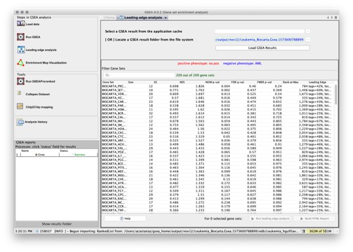
By default, gene sets are ordered by normalized enrichment score (NES). Click a column heading to reorder the gene sets based on the values in that column. For descriptions of the columns, see Interpreting GSEA Results.

By default, all gene sets are displayed. Use the filter box to display a subset of gene sets. As you enter text in the field, GSEA updates the list of gene sets to show only those that match the entered text. To change the text search options, click the magnifying class icon in the filter box.

4. Select one or more gene sets for the leading edge analysis. To select multiple gene sets, use SHIFT-click or CTRL-click.

5. Click Run leading edge analysis or Build HTML Report to start the analysis:

   • Run leading edge analysis displays four graphs that help you visualize the overlap between the selected leading edge subsets. (Does not generate an analysis results report.)
   • Build HTML Report creates an analysis results report that provides details on the leading edge subsets and the overlap between them. (Does not display the graphs.)

   If you are building an HTML report: track analysis progress, as described in Tracking Analysis Progress, and view analysis results, as described in Viewing Analysis Results.

6. Interpret analysis results, as described in Interpreting Leading Edge Analysis Results.

Running Other GSEA Analyses#

The GSEA application also provides the following analyses:

• Chip2Chip. Converts the genes in a gene set from the chip target namespace (eg. the “Gene Symbol” column to the identifiers in the “Probe Set ID” column for a selected target chip. For example, you can use this utility to convert MSigDB gene sets from HGNC gene symbols to probe identifiers for the HG_U95 microarray using the Human_AFFY_HG_U95_MSigDB.vX.chip.
• GSEAPreranked. Runs the gene set enrichment analysis against a ranked list of genes, which you supply. This provides an alternative method to the standard GSEA (Run GSEA icon), which ranks the genes in your expression dataset (based on the metric that you select using the metric for ranking genes parameter) and then analyzes that ranked list of genes.
• CollapseDataset. Creates a new dataset by collapsing each probe set into a single vector for the gene, which is identified by its HGNC gene symbol. When you run the gene set enrichment analysis with the Collapse dataset to gene symbols parameter set to True, GSEA runs this analysis as part of the gene set enrichment analysis.

To run one of these analyses:

1. Select the analysis from the Tools pane in the main GSEA window. The page for the selected analysis appears.
2. Enter values for the analysis parameters. For parameter descriptions, click Help, which displays the Chip2Chip, GSEAPreranked, or CollapseDataset page of this guide.
3. Click Run to start the analysis.
4. Track analysis progress, as described in Tracking Analysis Progress.
5. View analysis results, as described in Viewing Analysis Results.

Tracking Analysis Progress#

When you start an analysis, the gene set enrichment analysis or any other analysis, the Processes area in the bottom left corner of the window shows the analysis as running (blue). When the analysis is finished, it shows the analysis has succeeded (green). If an error occurs, it shows an error message (red). When you exit from GSEA, the Processes area is cleared.

1. Click Success to display analysis results in a web browser.
2. Click Error to display the error report. If you need help resolving the error, send us a description of the problem and the text of this error report via our help forum at groups.google.com/group/gsea-help.
3. Running – Displayed when an analysis is ongoing. Clicking the label in this state has no effect.
4. Click the analysis name to display the parameters used for the analysis. GSEA displays a page similar to the one you used to initially run the analysis. From this page, you can re-run the same analysis or modify the parameters to run a different analysis.
5. Click the status bar at the bottom of the window to display the execution log file.

Rerunning an Analysis#

To rerun an analysis:

1. From the Analysis History page, select the analysis that you want to re-run.

2. If you want to reload the data for this analysis, check that the Load Data box is selected.

   An analysis can only be run on data that you have loaded during the current session (see Loading Data). If you have not yet loaded the data from this analysis and this is the data that you want to analyze, reload it. If you have already loaded the data, or you want to rerun the analysis with other data that you have already loaded, you do not need to reload data.

3. Click Show in ToolRunner.

   GSEA displays a page similar to the one you used to initially run the analysis. From this page, you can leave the parameters unchanged to re-run the same analysis against the same data, or you can modify the parameters.

Note: When you analyze multiple gene sets, it is important to correct for multiple hypotheses testing. GSEA does this using sample permutation. Because of the random numbers used for sample permutation, when you rerun an analysis using the same data files and parameters, your results will be similar but not identical. Similarly, changing the order of the phenotypes does not affect analysis results, however, if you change the order of the phenotypes and rerun the analysis, your results will be similar but not identical because of the random numbers used for sample permutation.

Viewing Analysis Results#

When an analysis completes, GSEA updates the Processes area to show an analysis status of Success. To view the analysis results in a web browser, click the Success status.

Alternatively, you can use the Analysis History page to view the results of any previously run analysis:

• Displaying the Analysis History Page
• Setting the Default Output Folder
• Sharing Analysis Results
• Deleting Analysis Results

Displaying the Analysis History Page#

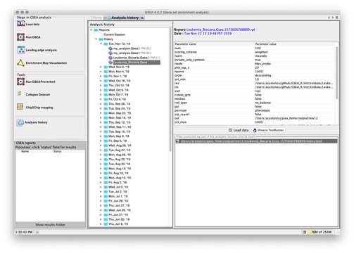
To display the Analysis History page, click the Analysis history icon in the GSEA main window. The Analysis History page displays all analysis results. The left side of the page lists analyses that you have run, organized by date. Select an analysis to display its parameters and generated files.

To view analysis results, double-click the index.html file in the list of files produced by the analysis. GSEA displays the results file in a web browser. Alternatively, select any file produced as part of the analysis and then right-click in the area. From the menu that appears, select the tool that you want to use to open the file.

Setting the Default Output Folder#

The Analysis History page displays all analysis results that are in the default output folder (Help>Show GSEA output folder). Your analysis results are in this folder unless you have taken one of the following actions:

• When you run an analysis, you can choose a location for the analysis results. If you chose an output folder, the analysis results are stored in that folder rather than in the default output folder.
• You can change the folder used as the default output folder by selecting Files>Preferences (see Preferences Window). If you changed the default output folder, analysis results stored in the original output folder are still in that folder unless you moved them.

The default output folder contains a subfolder named with today’s date (mmmdd, e.g. jan03). When you run an analysis, by default, GSEA creates a report subfolder in today’s output folder and writes all analysis results to that report subfolder. The report subfolder contains: - the analysis report (index.html) - the files linked to that report - a subfolder named edb that contains a machine-readable version of the report

Sharing Analysis Results#

To share analysis results with a colleague:

1. Select Help>Show GSEA output folder. GSEA displays the default reports output folder in a file browser.
2. Locate the report subfolder for the analysis whose results you want to share. Analyses are stored in subfolders named by the date when the analysis was run. If you are looking for an analysis that you previously ran, first go up one level in the folder hierarchy and then down into the folder for the date of interest.
3. Create a copy of that folder for your colleague. The analysis report (index.html) and the links to related files are preserved when you copy the folder.

Alternatively, when you run a gene set enrichment analysis, you can use the Make a zipped file with all reports parameter to create a zip file that contains the analysis results. If you chose to do so, you can share the analysis results by sending the zip file to your colleague. The zip file is saved in the report subfolder with all of the other analysis results.

Deleting Analysis Results#

When GSEA writes analysis results to an output folder, it also creates a matching .rpt file in the gsea_home/reports_cache folder (Help>Show GSEA home folder). The Analysis History page displays analysis results based on the .rpt files.

To delete analysis results:

1. Locate the matching .rpt file in the gsea_home/reports_cache folder. This file lists the analysis parameters and the full path name of the report output folder.
2. To delete the analysis results, delete the report output folder listed in the .rpt file.
3. To remove the analysis results from the Analysis History page, delete the .rpt file from the gsea_home/reports_cache folder. To update the Analysis History page, restart GSEA.

---

Interpreting GSEA Results#

This section discusses the results of the gene set enrichment analysis:

• GSEA Statistics
• GSEA Report

GSEA Statistics#

GSEA computes four key statistics for the gene set enrichment analysis report:

• Enrichment Score (ES)
• Normalized Enrichment Score (NES)
• False Discovery Rate (FDR)
• Nominal P Value

Enrichment Score (ES)#

The primary result of the gene set enrichment analysis is the enrichment score (ES), which reflects the degree to which a gene set is overrepresented at the top or bottom of a ranked list of genes. GSEA calculates the ES by walking down the ranked list of genes, increasing a running-sum statistic when a gene is in the gene set and decreasing it when it is not. The magnitude of the increment depends on the correlation of the gene with the phenotype. The ES is the maximum deviation from zero encountered in walking the list. A positive ES indicates gene set enrichment at the top of the ranked list; a negative ES indicates gene set enrichment at the bottom of the ranked list.

In the analysis results, the enrichment plot provides a graphical view of the enrichment score for a gene set:

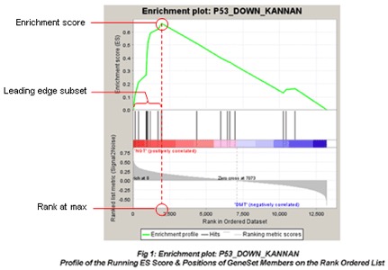
• The top portion of the plot shows the running ES for the gene set as the analysis walks down the ranked list. The score at the peak of the plot (the score furthest from 0.0) is the ES for the gene set. Gene sets with a distinct peak at the beginning (such as the one shown here) or end of the ranked list are generally the most interesting.

• The middle portion of the plot shows where the members of the gene set appear in the ranked list of genes. The leading edge subset of a gene set is the subset of members that contribute most to the ES. For a positive ES (such as the one shown here), the leading edge subset is the set of members that appear in the ranked list prior to the peak score. For a negative ES, it is the set of members that appear subsequent to the peak score.

• The bottom portion of the plot shows the value of the ranking metric as you move down the list of ranked genes. The ranking metric measures a gene’s correlation with a phenotype. The value of the ranking metric goes from positive to negative as you move down the ranked list. A positive value indicates correlation with the first phenotype and a negative value indicates correlation with the second phenotype. For continuous phenotypes (time series or gene of interest), a positive value indicates correlation with the phenotype profile and a negative value indicates no correlation or inverse correlation with the profile.

Note: By default, the ranking metric is the signal-to-noise ratio. To have GSEA rank the genes based on a different metric, use the Metric for ranking genes parameter of the Run GSEA Page. To have GSEA analyze a ranked list of genes that you have created, use the GSEAPreranked Page.

Normalized Enrichment Score (NES)#

The normalized enrichment score (NES) is the primary statistic for examining gene set enrichment results. By normalizing the enrichment score, GSEA accounts for differences in gene set size and in correlations between gene sets and the expression dataset; therefore, the normalized enrichment scores (NES) can be used to compare analysis results across gene sets. GSEA determines NES as follows:

NES is based on the gene set enrichment scores for all dataset permutations; therefore, changing the permutation method, the number of permutations, or the size of the expression dataset affects the NES. As an example, consider two analyses: (1) you analyze an expression dataset, GSEA generates a ranked list and analyzes that ranked list; (2) you use GSEAPreranked to analyze the ranked list generated by the first analysis. If you use the same parameter settings, your enrichment scores are identical; however, the normalized enrichment scores reflect the very different datasets (the expression dataset versus the ranked list of genes) used for the permutations:

	Expression Dataset		Ranked List
Gene Set Name	ES	NES	ES	NES
BRENTANI_DNA_MET_AND_MOD	0.1233649	0.37071982	0.1233649	0.42405358
BRCA_BRCA1_NEG	0.13040805	0.6497973	0.13040808	0.6497975
PENG_RAPAMYCIN_DOWN	0.14286387	0.84542555	0.14286387	0.76681024
BASSO_REGULATORY_HUBS_SET	0.14299561	0.6870111	0.14299563	0.69177157
VENTRICLES_UP	0.14565612	0.7033464	0.14565612	0.6915998
ALANINE_AND_ASPARTATE_METABOLISM	0.14693332	0.422703	0.14693332	0.36949828
BRCA1_OVEREXP_DN	0.15077576	0.7929205	0.15077576	0.68026066

Analysis parameters: P53_hgu95av2.gct, P53.cls#MUT_versus_WT, c2.may_2006.symbols.gmt, permutation type = gene_set, seed for permutation = 149, number of permutations = 10

False Discovery Rate (FDR)#

The false discovery rate (FDR) is the estimated probability that a gene set with a given NES represents a false positive finding. For example, an FDR of 25% indicates that the result is likely to be valid 3 out of 4 times. The GSEA analysis report highlights enrichment gene sets with an FDR of less than 25% as those most likely to generate interesting hypotheses and drive further research, but provides analysis results for all analyzed gene sets. In general, given the lack of coherence in most expression datasets and the relatively small number of gene sets being analyzed, an FDR cutoff of 25% is appropriate. However, if you have a small number of samples and use gene_set permutation (rather than phenotype permutation) for your analysis, you are using a less stringent assessment of significance and would then want to use a more stringent FDR cutoff, such as 5%.

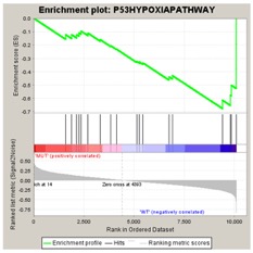
The FDR is a ratio of two distributions: (1) the actual enrichment score versus the enrichment scores for all gene sets against all permutations of the dataset and (2) the actual enrichment score versus the enrichment scores of all gene sets against the actual dataset. For example, if you analyze four gene sets and run 1000 permutations, the first distribution contains 4000 data points and the second contains 4. For an example of what the enrichment score for a permutation of the dataset might look like, consider the two enrichment plots shown below. The plot on the left shows actual enrichment results for the P53HYPOSIAPATHWAY gene set against the P53 dataset. The plot on the right shows enrichment results for that gene set against a phenotype permutation of the dataset (that is, when phenotype labels are randomly assigned to the samples).

Generally speaking, the larger the absolute NES the smaller the FDR; that is, as the absolute NES decreases the corresponding FDR increases. However, because the distribution curves tend to be “bumpy” at the tails, you may notice exceptions to this in your GSEA results. For similar reasons, although FDR is less conservative than FWER, you may notice instances in the GSEA results where the FWER is less than FDR.

The Gene Set Enrichment Analysis PNAS paper describes the FDR statistic in the section titled Appendix: Mathematical Description of Methods. For a more detailed discussion of the FDR, including a comparison with the more conservative familywise-error rate (FWER) statistic, see Benjamini and Hochberg (1995).

Nominal P Value#

The nominal p value estimates the statistical significance of the enrichment score for a single gene set. However, when you are evaluating multiple gene sets, you must correct for gene set size and multiple hypothesis testing. Because the p value is not adjusted for either, it is of limited value when comparing gene sets. The Gene Set Enrichment Analysis PNAS paper describes the p value statistic in the section titled Appendix: Mathematical Description of Methods.

The FDR is adjusted for gene set size and multiple hypotheses testing while the p value is not. When a top gene set has a small nominal p value and a high FDR value, it generally indicates that it is not as significant when compared with other gene sets in the empirical null distribution. This could be because you do not have enough samples, the biological signal is subtle, or the gene sets do not represent the biology in question very well. On the other hand, the FDR is based on two distributions of all gene sets; if only one of many gene sets is enriched, that gene set is likely to have a high FDR. Finally, a top gene set with a high nominal p value and a low FDR value, generally indicates a negative result: the gene set itself is not significant and other sets are weaker.

In the GSEA report, a p value of zero (0.0) indicates an actual p value of less than 1/number-of-permutations. For example, if the analysis performed 100 permutations, a reported p value of 0.0 indicates an actual p value of less than 0.01. For a more accurate p value, increase the number of permutations performed by the analysis. Typically, you will want to perform 1000 permutations (phenotype or gene_set). (If you attempt to perform significantly more than 1000 permutations, GSEA may run out of memory.)

GSEA Report#

This section discusses the content of the report generated by the gene set enrichment analysis:

• Enrichment in Phenotype
• Dataset Details
• Gene Set Details
• Gene Markers
• Global Statistics and Plots
• Other
• Detailed Enrichment Results
• Gene Set Details Report

Enrichment in Phenotype#

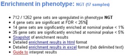
The analysis report contains two “Enrichment in Phenotype” sections. The first section shows results for gene sets that have a positive enrichment score (gene sets that show enrichment at the top of the ranked list) and the second section shows results for gene sets that have a negative enrichment score (gene sets that show enrichment at the bottom of the ranked list). For categorical phenotypes, a positive enrichment score indicates correlation with the first phenotype and a negative enrichment score indicates correlation with the second phenotype. For continuous phenotypes (time series or gene of interest), a positive value indicates correlation with the phenotype profile and a negative value indicates no correlation or inverse correlation with the phenotype profile.

For each phenotype, the report shows:

• Number of gene sets enriched in this phenotype and the total number of gene sets analyzed.
• Number of enriched gene sets that are significant, as indicated by a false discovery rate (FDR) of less than 25%. Typically, these are the gene sets most likely to generate interesting hypotheses and drive further research.
• Number of enriched gene sets with a nominal p value of less than 1% and of less than 5%. The nominal p value is not adjusted for gene set size or multiple hypothesis testing; therefore, it is of limited value for comparing gene sets.
• Snapshot of top results. Displays enrichment plots for the gene sets with the highest absolute normalized enrichment scores. By default, GSEA displays plots for the top 20 gene sets. To display a different number of plots, use the Plot graphs for the top sets of each phenotype parameter on the Run GSEA Page. For a description of the enrichment plot, see Enrichment Score (ES).
• Detailed enrichment results provide a summary report of gene sets enriched in this phenotype (html and excel formats).
• Guide to interpret results displays this section of the documentation.

The number of enriched gene sets depends on the structure of the data and the problem space. In general, one would expect to see at least a few gene sets enriched for a typical morphological or tissue-specific phenotype. If no enriched gene sets or a very large number of enriched gene sets pass the FDR threshold, first check that your gene sets and expression dataset use the same array format (see Consistent Feature Identifiers Across Data Files) and that you have used the appropriate permutation type and number of permutations (see the Run GSEA Page). If you find no issues, consider the following:

• No enriched gene sets of significance may indicate that, in fact, no gene sets are enriched. It may also be that you are analyzing too few samples, the biological signal in question is subtle, or the gene sets that you are analyzing do not represent the biology in question very well. You may still want to look at the top ranked gene sets, keeping in mind that these results provide weak evidence for potentially interesting hypotheses. You might also want to consider analyzing other gene sets or, if possible, additional samples.
• Too many enriched gene sets of significance may indicate that, in fact, many gene sets are enriched between phenotypes. Perhaps the gene sets represent the same biological signal. You can check for this by looking for overlap in the leading-edge subsets within the gene sets (see Running a Leading Edge Analysis). Or, you might be seeing significant differences between the phenotypes due to technical artifacts, such as samples being run in different labs, by different operators, or against different arrays. As with too few enriched gene sets, you may still want to look at the top ranked gene sets, keeping in mind that these results provide potentially biased evidence for interesting hypotheses. You might also want to consider analyzing other gene sets or, if possible, additional samples.

Dataset Details#

The Dataset Details section of the analysis report provides information about the expression dataset:

• Number of features (genes or probes) in the dataset.
• Number of genes in the dataset after collapsing each probe set into a gene (as shown above) or a note indicating that the probe sets were not collapsed (as shown below). For more information, see the Collapse dataset to gene symbols parameter on the Run GSEA Page.

Gene Set Details#

The Gene Set Details section of the analysis report provides information about the gene sets:

• Number of gene sets filtered out of the analysis due to size, and the minimum and maximum gene set sizes used for the filter.
• Number of gene sets used in the analysis.
• List of analyzed gene sets. For each gene set, the report shows the original number of genes in the gene set, the number of genes in the gene set after filtering out those genes not in the expression dataset, and the status of the gene set. Status is either blank (the gene set was included in the analysis) or “Rejected” (the gene set was filtered out of the analysis).

Note: If all gene sets are filtered out, the analysis fails. Typically, this occurs for one of the following reasons:

• The feature identifiers used for the expression dataset do not match those used in the gene sets. For example, your expression dataset contains probe identifiers from the HG_U133A chip and your gene sets identify genes based on HGNC gene symbols. For more information, see Consistent Feature Identifiers Across Data Files.
• After filtering out those genes not in the expression dataset, all of the gene sets are either larger than the maximum or smaller than the minimum gene set size allowed. You can use the Max Size and Min Size parameters on the Run GSEA Page to change the maximum and minimum gene set size.

Gene Markers#

The Gene Markers section of the analysis report provides information about the ranked list of genes used for the analysis:

• Number of features (genes or probes) in the dataset.
• Number of markers for each phenotype in the dataset; that is, the number of genes correlated with each phenotype. The bottom portion of the enrichment plot presents a graphical view of this information. For a description of the enrichment plot, see Enrichment Score (ES).
• Rank ordered list of genes in the dataset (Excel format), which includes the following information for each gene: probe, description, gene symbol, gene title, and rank metric score. The columns in this table are similar to those in the Gene Set Details Report.
• Heat map of the top 50 features for each phenotype and a plot showing the correlation between the ranked genes and the phenotypes. In a heat map, expression values are represented as colors, where the range of colors (red, pink, light blue, dark blue) shows the range of expression values (high, moderate, low, lowest).
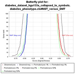
• Butterfly plot showing the positive and negative correlation between gene rank and the ranking metric score. By default, the butterfly plot shows the top 100 genes; that is, the first and last 100 genes in the ranked list. You can use the Number of markers parameter on the Run GSEA Page to change the number of genes displayed.

The bottom portion of the enrichment plot shows the observed correlation between gene rank and the ranking metric score for all genes in the ranked list. The butterfly plot shows the observed correlation, as well as permuted (1%, 5%, 50%) positive and negative correlation, for the top genes. The butterfly plot offers one way to visualize the extent to which dataset permutations change the correlation between gene rank and the ranking metric score.

Global Statistics and Plots#

The Global Statistics and Plots section provides additional information about the gene sets and enrichment results:

• Plot of p values versus normalized enrichment scores, which provides a quick, visual way to grasp the number of enriched gene sets that are significant.
• Histogram of enrichment scores across gene sets, which provides a quick, visual way to grasp the number of enriched gene sets.

Other#

The final section of the report, Other, lists the analysis parameters. Knowing the parameters is critical for reproducing analysis results.

Detailed Enrichment Results#

From the Enrichment in Phenotype section of the analysis report, you can click a link to display the detailed enrichment results report, which lists all gene sets enriched in this phenotype ordered by the normalized enrichment score (NES):

GS	Gene set name. Click the gene set name for a detailed description of the gene set. For MSigDB gene sets, the description is the gene set page on the GSEA website. For other gene sets, the description is provided by the author of the gene set.
GS DETAILS	For the top 20 gene sets, click the Details link to display the Gene Set Details Report. To generate the Details link for a different number of gene sets, use the Plot graphs for the top sets of each phenotype parameter on the Run GSEA Page.
SIZE	Number of genes in the gene set after filtering out those genes not in the expression dataset.
ES	Enrichment score for the gene set; that is, the degree to which this gene set is overrepresented at the top or bottom of the ranked list of genes in the expression dataset.
NES	Normalized enrichment score; that is, the enrichment score for the gene set after it has been normalized across analyzed gene sets.
NOM p-value	Nominal p value; that is, the statistical significance of the enrichment score. The nominal p value is not adjusted for gene set size or multiple hypothesis testing; therefore, it is of limited use in comparing gene sets.
FDR q-value	False discovery rate; that is, the estimated probability that the normalized enrichment score represents a false positive finding.
FWER p-value	Familywise-error rate; that is, a more conservatively estimated probability that the normalized enrichment score represents a false positive finding. Because the goal of GSEA is to generate hypotheses, the GSEA team recommends focusing on the FDR statistic.
RANK AT MAX	The position in the ranked list at which the maximum enrichment score occurred. The more interesting gene sets achieve the maximum enrichment score near the top or bottom of the ranked list; that is, the rank at max is either very small or very large.
LEADING EDGE	Displays the three statistics used to define the leading edge subset. Tags. The percentage of gene hits before (for positive ES) or after (for negative ES) the peak in the running enrichment score. This gives an indication of the percentage of genes contributing to the enrichment score. List. The percentage of genes in the ranked gene list before (for positive ES) or after (for negative ES) the peak in the running enrichment score. This gives an indication of where in the list the enrichment score is attained. Signal. The enrichment signal strength that combines the two previous statistics: where N is the number of genes in the list and Nh is the number of genes in the gene set. If the gene set is entirely within the first Nh positions in the list, then the signal strength is maximal or 100%. If the gene set is spread throughout the list, then the signal strength decreases towards 0%. These statistics describe the leading-edge subset of a single gene set. Use the Leading Edge analysis to analyze the overlap between multiple leading-edge subsets.

Gene Set Details Report#

From the Detailed Enrichment Results table, click the Details link for a gene set to display a Gene Set Details report that contains the following:

• A table showing the GSEA results for this gene set. The fields in this table are similar to those in the Detailed Enrichment Results.
• An enrichment plot for this gene set, as described in Enrichment Score (ES).
• A table of genes in the gene set ordered by their position in the ranked list of genes. The analysis includes only those genes in the gene set that are also in the expression dataset. To display the table in Excel, click the plain text format link in the table header.

---

Interpreting Leading Edge Analysis Results#

When you click Run leading edge analysis on the Leading Edge Analysis Page, GSEA displays four graphs that help you visualize the overlap between the selected leading edge subsets. When you click Build HTML Report, GSEA generates an analysis results report that provides details on the leading edge subsets and the overlap between them. This section describes each graph and then the report:

• Heat Map
• Set-to-Set
• Gene in Subsets
• Histogram
• HTML Report

Heat Map#

The heat map shows the (clustered) genes in the leading edge subsets. In a heat map, expression values are represented as colors, where the range of colors (red, pink, light blue, dark blue) shows the range of expression values (high, moderate, low, lowest).

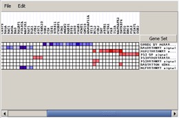
• Use the File menu to save the dataset or the heat map image.
• Use the Edit menu to change the grid size of the heat map. Decrease the grid size to zoom out.
• Hover over a cell to display the associated gene and gene set names.

Set-to-Set#

The top right graph uses color intensity to show the overlap between subsets: the darker the color, the greater the overlap between the subsets. Specifically, the intensity of the cell for sets A and B corresponds to an X/Y ratio where X is the number of leading edge genes from set A and Y is the union of leading edge genes in sets A and B. A dark green cell indicates that sets A and B have the same leading edge genes and a white cell indicates that sets A and B have no leading edge genes in common.

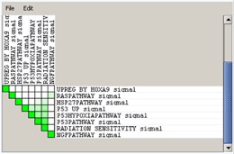
• Use the File menu to save the dataset or the image.
• Use the Edit menu to change the grid size of the graph. Decrease the grid size to zoom out.

Gene in Subsets#

The bottom left graph shows each gene and the number of subsets in which it appears.

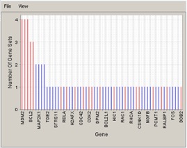
• Use the File menu to save or print the image.
• Use the View menu to zoom in, zoom out, or change the look of the graph (add a title, change the label and look of the axes, or the color of the background).

Histogram#

The last plot is a histogram, where the Jacquard is the intersection divided by the union for a pair of leading edge subsets. Number of Occurrences is the number of leading edge subset pairs in a particular bin. In this example, most subset pairs have no overlap (Jacquard = 0).

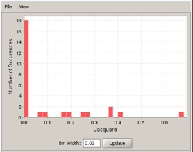
• Use the File menu to save or print the image.
• Use the View menu to zoom in, zoom out, or change the look of the histogram (add a title, change the label and look of the axes, or the color of the background).

HTML Report#

The HTML Report for the leading edge analysis contains the following sections:

• Clustered results. Provides the number of gene sets analyzed and a heat map of the leading edge subsets after clustering.

• Details of gene sets. Provides the following information for each of the analyzed gene sets and its leading edge subset:

  • # members. Number of genes in the gene set.
  • # members in signal. Number of genes in the leading edge subset.
  • Tag %. The percentage of gene hits before (for positive ES) or after (for negative ES) the peak in the running enrichment score. This gives an indication of the percentage of genes contributing to the enrichment score.
  • List %. The percentage of genes in the ranked gene list before (for positive ES) or after (for negative ES) the peak in the running enrichment score. This gives an indication of where in the list the enrichment score is attained.
  • Signal strength. The enrichment signal strength that combines the two previous statistics:

  

  where N is the number of genes in the list and Nh is the number of genes in the gene set. If the gene set is entirely within the first Nh positions in the list, then the signal strength is maximal or 100%. If the gene set is spread throughout the list, then the signal strength decreases towards 0%.

• Other files made. Provides a heat map of the (unclustered) leading edge subsets and tabular ways of examining the leading edge subsets:

  • Clustered dataset (gct) uses the expression dataset format to describe the clustered leading edge subsets: each row is a gene set, each column is a gene, and an “expression value” of 1 indicates the gene is in the leading edge subset for the gene set.
  • GeneMatrix (gms) provides a gene set file for the leading edge subsets, which lists each gene set and the genes in its leading edge subset.
  • Dataset (gct) uses the expression dataset format to describe the leading edge subsets (not clustered): each row is a gene set, each column is a gene, and an “expression value” of 1 indicates the gene is in the leading edge subset for the gene set.
  • Heat map shows a heat map of the leading edge subsets (not clustered).
• Other. Lists the analysis parameters. Knowing the parameters used to produce the analysis is critical for reproducible research.

---

Running GSEA from the Command Line#

GSEA is most commonly used by running the GSEA desktop application that provides the user interface for controlling the analyses. However, you can also run GSEA from the command line. This can be useful, for example, when you want to analyze several datasets at once or analyze a large dataset, or a large number of gene sets, on a server or compute cluster.

• Syntax
• Output
• Examples

Syntax#

To run GSEA from the command line, download the “GSEA for the command line (all platforms)” zip bundle from the website and use either the gsea-cli.sh (Mac and Linux) or gsea-cli.bat (Windows) script. Note that this bundle requires the user to have the correct version of Java installed and available. The required Java version is noted on the Downloads page of the website. The “GSEA for Linux” zip bundle also contains the gsea-cli script along with an embedded platform-specific copy of Java.

Use a command of the form: gsea-cli.sh operation-name parameters

operation-name

Specifies the analysis to use. One of: GSEA, GSEAPreranked, CollapseDataset, Chip2Chip, or LeadingEdgeTool

parameters

Specifies the analysis parameters. To find the parameters for an analysis, open the GSEA desktop application, display the page that runs the analysis, enter the parameters that you want to use, and click the Command button at the bottom of the page. GSEA displays the command line used to run the analysis. If you omit a parameter, GSEA uses the default value as displayed in the GSEA application. Paths to file names must be fully specified or relative to the execution directory. When creating batch files, you generally want to use full path names for all files. File names are platform-specific and may require editing. For example, on Windows, a file name that contains spaces must be enclosed in quotation marks. Files cannot be directly referenced from the GSEA-MSigDB file servers. Download the desired gene set or array annotations files from the GSEA website downloads page and reference the downloaded files in the command line. Parameter values cannot include hyphens (-); therefore, file names cannot include hyphens. If necessary, change hyphens to underscores. For example, you cannot use -res my-dataset.gct, but can use -res my_dataset.gct instead. GSEA also has issues with parameter values containing spaces or other special characters. Optionally, use the –param_file parameter to specify a parameter file, which can contain any parameter except –param_file. If you specify the same parameter on the command line and in the parameter file, the value on the command line takes precedence. A parameter file is a text file that defines one parameter per line. Each line contains a parameter name (without the initial hyphen), a tab (not spaces), and the parameter value. Note: The Leading Edge Analysis Page does not include a Command button; therefore, the command line syntax for building a leading edge HTML report is provided here: gsea-cli.sh LeadingEdgeTool -dir path_to_gsea_report_dir -gsets set_names_comma_delimited

For very large analyses, the GSEA default memory specification might not be sufficient. You can increase the memory available to GSEA by editing the gsea-cli script and changing the -Xmx4g parameter to a larger value (alternatively, on memory-constrained machines it might be necessary to reduce this value). The default specifies 4 GB of memory, so change this to -Xmx8g for 8 GB or -Xmx2g for 2 GB, for example.

Only edit the script with a plain-text editor (such as TextEdit.app on Mac, emacs or vi on Linux, or NotePad on Windows). Be sure to save the file as plain-text only, no matter which editor you use.

Output#

By default, the GSEA command line writes analysis reports to a dated subfolder, mmmdd, in the current working directory. To write analysis reports to a different location, use the –out parameter. (GSEA will still create the mmmdd subfolder in the current directory, but writes the reports to the specified location.) To specify a report name, rather than using the default name of my_analysis, use the -rpt_label parameter.

Note: The GSEA application uses a different graphical imaging package than the GSEA command line; therefore, heat maps generated from the GSEA command line look different from heat maps generated by the GSEA application.

Examples#

1. Following is a command line that might appear when you click the Command button in GSEA. In this example, the –gmx and –chip parameters reference files hosted on the GSEA-MSigDB file servers. You must download these files from the GSEA website and update the command line to reference the downloaded files. If necessary, quote file names that include spaces and/or remove hyphens from the file names.

   gsea-cli.sh GSEA

   -res P53_hgu95av2.gct -cls P53.cls#MUT_versus_WT -gmx c1.v2.symbols.gmt -chip HG_U95Av2.chip

   -collapse true -mode Max_probe -norm meandiv -nperm 1000 -permute phenotype

   -rnd_type no_balance -scoring_scheme weighted -rpt_label my_analysis

   -metric Signal2Noise -sort real -order descending -include_only_symbols true

   -make_sets true -median false -num 100 -plot_top_x 20 -rnd_seed timestamp

   -save_rnd_lists false -set_max 500 -set_min 15 -zip_report false

   -out dec18 -gui false

2. Following is a command line that assumes that the identifiers in your dataset match those in your gene sets:

   gsea-cli.sh GSEA -res test.gct -cls test.cls -gmx test.gmx -collapse false

3. Following is a command line that assumes that your dataset uses HG_U133A probe identifiers and your gene sets use gene symbols, so you want to collapse your dataset:

   gsea-cli.sh GSEA -res foo.gct -cls foo.cls -gmx foo.gmx -chip HG_U133A.chip

---

Quick Reference#

This section provides descriptions of the GSEA menu bar and windows:

• Menu Bar
• GSEA Main Window
• Load Data Page
• Run GSEA Page
• Leading Edge Analysis Page
• Chip2Chip Page
• Analysis History Page
• GSEAPreranked Page
• CollapseDataset Page
• Preferences Window

Menu Bar#

File#

• Preferences. Displays the Preferences Window, which allows you to set GSEA configuration options.
• Clear recent file history. Removes all files from the Recently Used Files pane of the Load Data Page.

Downloads#

• Download chip annotations. Displays the DNA chip (array) annotations files available on the GSEA website.
• Download example datasets. Displays the example datasets available on the GSEA website.

Help#

• GSEA website. Displays the home page of the GSEA website.
• GSEA documentation. Displays the documentation page of the GSEA website.
• GSEA & MSigDB License Terms. Displays GSEA-MSigDB website page containing the terms under which the GSEA application and Molecular Signatures Database is licensed.
• Show GSEA home folder. Displays the gsea_home folder in a file browser. The gsea_home folder contains the default output folder and the reports_cache folder, as described in Viewing Analysis Results.
• Show GSEA output folder. Displays GSEA analysis results, as described in Viewing Analysis Results. By default, GSEA writes analysis results to this folder. To select a different folder, use the Preferences Window.
• Contact Us. Directs to the GSEA team contact information page, which includes information on how to reach us for questions, comments, or suggestions.
• The final item is GSEA build number and the date of the build. When reporting a problem, you may be asked for this information.

GSEA Main Window#

The GSEA main window appears when you start the GSEA desktop application. The one page open in the window is the Startup page. As you open new pages, tabs appear next to the Startup tab. To close a page, click the close (X) icon on the tab.

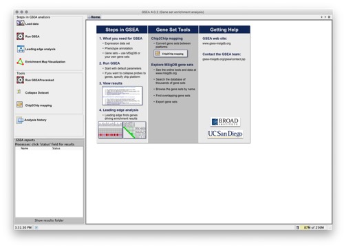
• Use the icons on the left for quick access to the primary GSEA operations:
  • Load Data Page
  • Run GSEA Page
  • Leading Edge Analysis Page
  • Run GSEAPreranked Page
  • Collapse Dataset Page
  • Chip2Chip Page
  • Analysis History Page
• Use the Processes area to track the status of analyses that you run, as described in Tracking Analysis Progress.
• For descriptions of the menu bar items, see Menu Bar.

Load Data Page#

Use the Load Data page to load data files into GSEA. You must load data files before you can analyze them. To display the Load Data page, select the Load Data icon in the GSEA main window. For more information, see Loading Data.

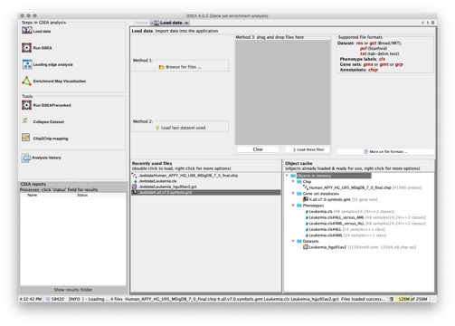
Run GSEA Page#

Use the Run GSEA page to run the gene set enrichment analysis. To display this page, click the Run GSEA icon in the GSEA main window.

Place your cursor on a parameter name to see a brief description of the parameter.

Required Fields lists parameters that are essential for the analysis. Enter values for these parameters before starting the analysis.

• Expression dataset. Select an expression dataset from the drop-down list. If the dataset is not listed, you have not yet loaded it; see Loading Data.
• Gene sets database. Click the ellipse (…) button and select one or more gene sets:
  • GeneMatrix (from website) lists the MSigDB gene sets hosted on the GSEA-MSigDB file servers. These gene set files may each contain hundreds of gene sets. See Exporting Gene Sets from MSigDB on how create gene set files containing only a subset of MSigDB gene sets of interest.
  • GeneMatrix (local gmx/gmt) lists the gene set files that you have loaded (see Loading Data).
  • GeneSets(grp) lists gene sets that GSEA has created in memory; for example, gene sets created using the Text Entry tab described below.
  • Subsets lists each gene set in each gmx/gmt file that you have loaded.
  • Text Entry allows you to create a gene set by entering the genes for that gene set; enter one gene per line. The gene set is deleted when you exit from GSEA.
• Number of permutations. Specify the number of permutations to perform in assessing the statistical significance of the enrichment score. It is best to start with a small number, such as 10. After the analysis completes successfully, run it again with a full set of permutations. The GSEA team recommends 1000 permutations.
• Phenotype labels. Click the ellipse (…) button to display the Select a Phenotype Window, which allows you to select a phenotype to analyze.

• Chip platform(s). Click the ellipse (…) button and select one or more DNA chip (array) annotation files:

  • Chips (from website) lists the chip annotation files hosted on the GSEA-MSigDB file servers.
  • Chips (local .chip) lists the chip annotation files that you have loaded (see Loading Data).

  This parameter is mandatory or optional depending on the value of the Collapse/Remap to gene symbols parameter.

• Collapse/Remap to gene symbols:

  • Select “Collapse” (default) to have GSEA collapse each probe set in the expression dataset into a single vector for the gene, which gets identified by its HGNC gene symbol. When you select “Collapse”, you must specify a chip annotation file (Chip platform parameter) and gene sets (Gene sets database parameter) that identify genes by the same namespace.
  • Select “Remap_Only” to have GSEA map each identifier in the expression dataset to its respective gene symbol. This operation does not perform any mathematical collapse and requires each input identifier to map uniquely to an output gene symbol. When you select “Remap_Only”, you must specify a chip annotation file (Chip platform parameter) and gene sets (Gene sets database parameter) that identify genes by the same namespace.
  • Select “No_Collapse” to use your expression dataset as is (with its native feature identifiers). When you select this option, the chip annotation file (Chip platform parameter) is optional and you must specify gene sets (Gene sets database parameter) that identify genes using the same feature (gene or probe) identifiers as those used in your expression dataset.

  For more information, see Consistent Feature Identifiers Across Data Files.

• Permutation type. Select the type of permutation to perform in assessing the statistical significance of the enrichment score:

  • Phenotype. Random phenotypes are created by shuffling the phenotype labels on the samples. For each random phenotype, GSEA ranks the genes and calculates the enrichment score for all gene sets. These enrichment scores are used to create a null distribution from which the significance of the actual enrichment score (for the actual expression data and gene set) is calculated. This is the recommended method when there are at least seven (7) samples in each phenotype.
  • Gene_set. Random gene sets, size matched to the actual gene set, are created and their enrichment scores calculated. These enrichment scores are used to create a null distribution from which the significance of the actual enrichment score (for the actual gene set) is calculated. This method is useful when you have too few samples to do phenotype permutations (that is, when you have fewer than seven (7) samples in any phenotype).

  The GSEA team recommends using phenotype permutation whenever possible. The phenotype permutation shuffles the phenotype labels on the samples in the dataset; it does not modify gene sets. Therefore, the correlations between the genes in the dataset and the genes in a gene set are preserved across phenotype permutations. The gene_set permutation creates random gene sets; therefore, the correlations between the genes in the dataset and the genes in the gene set are not preserved across gene_set permutations. Preserving the gene-to-gene correlation across permutations provides a more biologically reasonable (more stringent) assessment of significance.

Note: In previous versions of GSEA, gene_set permutation was referred to as tag permutation.

Basic Fields lists additional parameters with standard defaults. Typically, you use the default values for these parameters. Click Show/Hide to display and hide these parameters.

• Analysis name. A short descriptive label for the analysis. The name cannot include spaces. This label is used as a prefix when naming the output report generated by the analysis (for example, my_analysis.Gsea.1130510139575.rpt).
• Enrichment statistic. To calculate the enrichment score, GSEA first walks down the ranked list of genes increasing a running-sum statistic when a gene is in the gene set and decreasing it when it is not. The enrichment score is the maximum deviation from zero encountered during that walk. This parameter affects the running-sum statistic used for the analysis. The last section of the Gene Set Enrichment Analysis PNAS paper shows the mathematical descriptions of the methods used in GSEA. This option controls the value of p used in the enrichment score calculation shown there. Note that genes with infinite or NaN value scores will be adjusted to a score of 0.01 in the weighted mode or 0.000001 in the weighted_p2 and weighted_p1.5 modes.
  • classic: p=0
  • weighted (default): p=1
  • weighted_p2: p=2
  • weighted_p1.5: p=1.5
• Metric for ranking genes. GSEA ranks the genes in the expression dataset and then analyzes that ranked list of genes. Use this parameter to select the metric used to score and rank the genes; use the Gene list sorting mode parameter to determine whether to sort the genes using the real (default) or absolute value of the metric score; and use the Gene list ordering mode parameter to determine whether to sort the genes in descending (default) or ascending order. For descriptions of the ranking metrics, see Metrics for Ranking Genes.

Note: The default metric for ranking genes is the signal-to-noise ratio. To use this metric, your phenotype file must define at least two categorical phenotypes and your expression dataset must contain at least three (3) samples for each phenotype. If you are using a continuous phenotype or your expression dataset contains fewer than three samples per phenotype, you must choose a different ranking metric. If your expression dataset contains only one sample, you must rank the genes and use the GSEAPreranked Page to analyze the ranked list; none of the GSEA metrics for ranking genes can be used to rank genes based on a single sample.

• Gene list sorting mode. GSEA ranks the genes in the expression dataset and then analyzes that ranked list of genes. Use this parameter to determine whether to sort the genes using the real (default) or absolute value of the ranking metric.
• Gene list ordering mode. GSEA ranks the genes in the expression dataset and then analyzes that ranked list of genes. Use this parameter to determine whether to sort the genes in descending (default) or ascending order. Ascending order is usually applicable when the ranking metric is a measure of nearness (how close the genes are to one another) rather than distance.
• Max size. After filtering from the gene sets any gene not in the expression dataset, gene sets larger than this are excluded from the analysis.
• Min size. After filtering from the gene sets any gene not in the expression dataset, gene sets smaller than this are excluded from the analysis.
• Save results in this folder. Path of the directory in which to place the analysis results. Existing results in this folder are not overwritten. By default, analysis results are saved in the GSEA output folder. To view this folder, select Help>Show GSEA output folder.

Advanced Fields lists parameters that control details of the GSEA algorithm and its Java implementation. Do not change the default values of these parameters unless you are conversant with the algorithm and its Java implementation. Click Show/Hide to display and hide these parameters.

• Collapsing mode for probe sets => 1 gene. Used only when the Collapse/Remap to gene symbols parameter is set to “Collapse”. Select the expression values to use for the single identifier that will represent all identifiers for the gene:

  • Max_probe (default): for each sample, use the maximum expression value for the identifiers. For example:

  Probeset_A	10	20	15	200
  Probeset_B	100	105	110	95
  gene_symbol_AB	100	105	110	200

  • Median_of_probes: for each sample, use the median expression value for the identifiers.
  • Mean_of_probes: for each sample, use the mean expression value for the identifiers.
  • Sum_of_probes: for each sample, sum the values of the identifiers.
  • Abs_max_of_probes: for each sample, use the expression value with the maximum absolute vale for the identifiers. Note that each value retains its original sign but is chosen based on absolute value. In other words, the largest magnitude value is used. While this method is useful with computational-based input datasets — and thus is the default for GSEAPreranked — it is generally not recommended for use with quantification-based expression measures such as counts or microarray fluorescence.

• Normalization mode. Method used to normalize the enrichment scores across analyzed gene sets:

  • meandiv (default): GSEA normalizes the enrichment scores as described in Normalized Enrichment Score (NES).
  • none: GSEA does not normalize the enrichment scores.

• Randomization mode. Method used to randomly assign phenotype labels to samples for phenotype permutations. Not used for gene_set permutations.

  • no_balance (default). Permutes labels without regard to number of samples per phenotype. For example, if your dataset has 12 samples in class_a and 10 samples in class_b, any permutation of class_a has 12 samples randomly chosen from the dataset.
  • equalize_and_balance. Permutes labels by equalizing the number of samples per phenotype and then balancing the number of samples contributed by each phenotype. For example, if your dataset has 12 samples in class_a and 10 samples in class_b, any permutation of class_a has 10 samples: 5 randomly chosen from class_a and 5 randomly chosen from class_b.

  The GSEA team recommends using no_balance (default), unless the number of samples per phenotype is highly unbalanced.

• Alternate delimiter. Allows specifying an alternate character instead of comma when selecting individual gene sets in the Gene Sets Database selection. This is only necessary if the gene set names contain commas.

• Create GCT files. Allows saving the dataset subsets backing the GSEA report heatmaps as GCT files; these will be subsets of the original dataset corresponding only to the genes of the heatmap. These GCT files may be useful for subsequent analysis or visualization by other tools such as R, Python, GenePattern, etc.
• Create SVG plot images. Allows the creation of SVG images along with PNGs. Saving SVGs is CPU-intensive and requires a lot of storage; therefore this is set to false by default. They are GZ compressed for the same reason and can be decompressed using e.g. ‘gunzip’ on Mac and Linux and 7-Zip on Windows. Note that the SVG plots may match closely but not exactly to the PNGs. The fonts in particular may be slightly different.
• Omit features with no symbol match. Used only when Collapse/Remap to gene symbols is set to “Collapse” or “Remap_Only”. By default (true), the new dataset excludes probes/genes that have no gene symbols. Set to False to have the new dataset contain all probes/genes that were in the original dataset.
• Make detailed gene set report. Set to True (default) to create a detailed gene set report for each enriched gene set.
• Median for class metrics. Set to True (default=False) to use the median of each class, instead of the mean, in the metrics for ranking genes. The Use median instead of mean for metrics item in the Preferences controls the default setting for this parameter. (If you change the setting in the Preferences window, the new default takes effect the next time you start GSEA.)
• Number of markers. Number of features (gene or probes) to include in the butterfly plot in the Gene Markers section of the gene set enrichment report.
• Plot graphs for the top sets of each phenotype. Generates summary plots and detailed analysis results for the top x genes in each phenotype, where x is 20 by default. The top genes are those with the largest normalized enrichment scores.
• Seed for permutation. Seed used to generate a random number for phenotype and gene_set permutations: timestamp (default), 149, or user input. The specific seed value (149) generates consistent results, which is useful when testing software.
• Save random ranked lists. Set to True (default=false) to save the random ranked lists of genes created by phenotype permutations. When you save random ranked lists, for each permutation, GSEA saves the rank metric score for each gene (the score used to position the gene in the ranked list). Saving random ranked lists is memory intensive; therefore, this parameter is set to false by default.
• Make a zipped file with all reports. Set to True (default=false) to create a zip file of the analysis results. The zip file is saved to the output folder with all of the other files generated by the analysis. This is useful for sharing analysis results.

Buttons at the bottom of the page:

• Help. Displays this documentation.
• Reset. Restores the default values for all parameters.
• Last. Loads the data used the last time you ran this analysis.
• Command. Displays the command line used to run the analysis, as described in Running GSEA from the Command Line.
• Run. Starts the analysis.

Metrics for Ranking Genes#

When you run the gene set enrichment analysis from the Run GSEA Page, GSEA ranks the genes in the expression dataset and then analyzes that ranked list of genes. You use the Metric for ranking genes parameter to select the metric used to score and rank the genes; the Gene list sorting mode parameter to determine whether to sort the genes using the real (default) or absolute value of the metric score; and the Gene list ordering mode parameter to determine whether to sort the genes in descending (default) or ascending order.

This section describes each of the ranking metrics in the drop-down list of the Metric for ranking genes parameter. If your favorite metric is not listed here, you can rank the genes in your dataset using that metric and then use the GSEAPreranked Page to analyze your ranked list of genes. If your dataset contains only one sample, GSEA cannot rank the genes; however, you can rank the genes and then use the GSEAPreranked Page to analyze your ranked list of genes.

Three settings in the Algorithms tab of the Preferences window (selected from the File menu in the application menu bar) affect the calculations shown here:

• Use median instead of mean for metrics. For categorical phenotypes, by default, GSEA calculates differential expression based on the mean expression value for each phenotype. To use the median expression value for each phenotype, set the Median for class metrics parameter on the Run GSEA page to True. To always use the median expression value for each phenotype, click on the checkbox to enable the Use median instead of mean for class metrics option in the Preferences window. The new default value takes effect when you restart GSEA. By default, this option is not selected. Note: Using median rather than mean may cause ties in the ranking.
• Fix metrics for low variance. When calculating ranking metrics, the denominator may be zero (0). A denominator of zero (0) causes an error in the analysis unless this option is selected. By default, this option is selected.
• Use biased variances. When calculating ranking metrics, GSEA uses an unbiased variance to calculate standard deviation. Select this option to have GSEA use a biased variance instead. By default, this option is not selected.

For categorical phenotypes, GSEA determines a gene’s mean expression value for each phenotype and then uses one of the following metrics to calculate the gene’s differential expression with respect to the two phenotypes. To use median rather than mean expression values, set the Median for class metrics parameter to True, as described above.

• Signal2Noise (default) uses the difference of means scaled by the standard deviation. Note: You must have at least three samples for each phenotype to use this metric.

where μ is the mean and σ is the standard deviation; σ has a minimum value of .2 * absolute(μ), where μ=0 is adjusted to μ=1. The larger the signal-to-noise ratio, the larger the differences of the means (scaled by the standard deviations); that is, the more distinct the gene expression is in each phenotype and the more the gene acts as a “class marker.”

• tTest uses the difference of means scaled by the standard deviation and number of samples. Note: You must have at least three samples for each phenotype to use this metric.

where μ is the mean, n is the number of samples, and σ is the standard deviation; σ has a minimum value of .2 * absolute(μ), where μ=0 is adjusted to μ=1. The larger the tTest ratio, the more distinct the gene expression is in each phenotype and the more the gene acts as a “class marker.”

• Ratio_of_Classes (also referred to as fold change) uses the ratio of class means to calculate fold change for natural scale data:

where μ is the mean. The larger the fold change, the more distinct the gene expression is in each phenotype and the more the gene acts as a “class marker.”

• log2_Ratio_of_Classes uses the log2 ratio of class means to calculate fold change for natural scale data:

where μ is the mean. This is the recommended statistic for calculating fold change for natural scale data.

For continuous phenotypes, GSEA determines an ideal expression profile based on the phenotype (.cls) file, determines a gene’s expression profile based on the expression dataset (.gct) file, and then uses one of the following metrics to calculate the correlation between the two expression profiles. Note: You can also use these metrics to analyze categorical phenotypes: in your phenotype labels file, specify the categorical phenotype labels as numbers.

• Pearson uses Pearson's correlation to determine the degree of linear relationship between the two profiles, where +1 indicates a perfect positive relationship, 0 indicates no relationship, and -1 indicates a perfect inverse relationship.

Pearson is the only metric that does not require the two profiles to use the same unit of measure; therefore, Pearson is the only metric that can be used with a time series phenotype. For the same reason, of the continuous phenotype metrics, Pearson is the most useful for analyzing categorical phenotypes.

• Cosine is a variant of Pearson’s that is defined by Eisen et al. (1998). It is appropriate only when the expression profiles are based on log-expression ratios relative to a control.
• Manhattan measures similarity based on a distance measure, where the distance between two objects is given by the length of a line assuming that you can travel in only one direction at a time (imagine the points are on a grid and you must move vertically and horizontally, rather than diagonally, to move between them).
• Euclidean measures similarity based on a distance measure, where the distance between two objects is the length of a straight line between the objects.

Statistics reference: Statistics for Microarrays, Wit, E. and McClure J., John Wiley & Sons Ltd., 2004.

Select a Phenotype Window#

On the Run GSEA page, next to the Phenotype labels parameter, click the ellipse (…) button to display the following window, which allows you to select a phenotype to analyze.

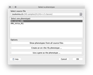
• Select source file. Select a phenotype labels file from the drop-down list. If you don’t see your file, make sure it has been loaded (see Loading Data). GSEA updates the window to display the phenotypes in the selected file. Select a phenotype to analyze and click OK.
• Show phenotypes from all source files. Updates the window to display all phenotypes from all loaded phenotype files (not phenotypes that you created using this window). Select a phenotype to analyze and click OK.
• Create an on-the-fly phenotype. Displays the following window, which allows you to create categorical phenotype labels:

1. Enter the names of one or more samples in the box on the left and enter a name for that phenotype class (by default, ClassA). For easier entering of sample names, cut and paste from your dataset file.
2. Enter the names of one or more samples in the box on the right and enter a name for that phenotype class (by default, ClassB). If your dataset contains samples not included in the two phenotypes, GSEA automatically excludes them from the gene set enrichment analysis of these phenotypes.
3. Select your dataset and click Apply to dataset. GSEA confirms that all of the samples that you specified are in the selected dataset and creates a phenotype labels file (ClassAvsClassB.cls) in the default output folder. When you close this window, the new phenotype labels file appears in the Select source file drop-down list of the Select a Phenotype window.

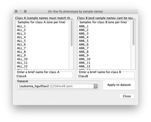
• Use a gene as the phenotype. Displays the following window, which allows you to create a continuous phenotype label to find gene set correlations with a gene of interest (gene neighbors). Select your dataset. GSEA updates the window to display the genes in the dataset. Select a gene and click Apply to dataset. GSEA confirms that the gene is in the selected dataset and creates a phenotype labels file (genename_in_datasetname.cls) in the default output folder. When you close this window, the new phenotype labels file appears in the Select source file drop-down list of the Select a Phenotype window.

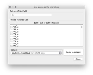
Leading Edge Analysis Page#

To display the Leading Edge Analysis page, select the Leading Edge Analysis icon in the GSEA main window. For more information, see Running a Leading Edge Analysis and Interpreting Leading Edge Analysis Results.

Chip2Chip Page#

The Chip2Chip analysis translates the gene identifiers in a gene sets from HGNC gene symbols to the probe identifiers for a selected DNA chip. If you prefer to analyze your dataset without collapsing the probe sets to gene symbols, you can use Chip2Chip to translate MSigDB gene sets to the required chip platform format (see Consistent Feature Identifiers Across Data Files).

To display the Chip2Chip page, select the Chip2Chip icon in the GSEA main window.

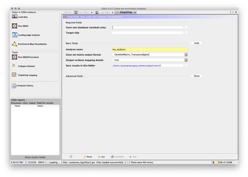
Place your cursor on a parameter name to see a brief description of the parameter.

Required Fields lists parameters that are essential for the analysis. Enter values for these parameters before starting the analysis.

• Gene sets database. Click the ellipse (…) button and select one or more gene sets; genes in the selected gene sets must be identified by HGNC gene symbol:
  • GeneMatrix (from website) lists the MSigDB gene sets hosted on the GSEA-MSigDB file servers. These gene set files may contain hundreds of gene sets. See Exporting Gene Sets from MSigDB on how create gene set files containing only a subset of MSigDB gene sets of interest.
  • GeneMatrix (gmx/gmt) lists the gene set files that you have loaded.
  • GeneSets(grp) lists gene sets that GSEA has created in memory; for example, gene sets created using the Text Entry tab described below.
  • Subsets lists each gene set in each gmx/gmt file that you have loaded.
  • Text Entry allows you to create a gene set by entering the genes for that gene set; enter one gene per line. The gene set is deleted when you exit from GSEA.
• Target chip. Click the ellipse (…) button and select one or more DNA chip (array) annotation files:
  • Chips (from website) lists the chip annotation files hosted on the GSEA-MSigDB file servers.
  • Chips (local .chip) lists the chip annotation files that you have loaded (see Loading Data).

Basic Fields lists additional parameters with standard defaults. Typically, you use the default values for these parameters. Click Show/Hide to display and hide these parameters.

• Analysis name. A short descriptive label for the analysis. The name cannot include spaces. This label is used as a prefix when naming the output report generated by the analysis (for example, my_analysis.Chip2Chip.1130510139575.rpt).
• Gene set database output format. Select a gene set file format for the new gene sets:
  • GeneSetMatrix_transposed [gmt] (default)
  • GeneSetMatrix [gmx]
• Output verbose mapping details. Set to True (default) to create a detailed report that lists the translation of each feature identifier in each gene set.
• Save results in this folder. Path of the directory in which to place the analysis results. Existing results in this folder are not overwritten. By default, analysis results are saved in the GSEA output folder. To view this folder, select Help>Show GSEA output folder.

Advanced Fields lists parameters that control details of the GSEA algorithm and its Java implementation. Do not change the default values of these parameters unless you are conversant with the algorithm and its Java implementation. Click Show/Hide to display and hide these parameters.

• Alternate delimiter.
• Make a zipped file with all reports. Set to True (default=false) to create a zip file of the analysis results. The zip file is saved to the GSEA output folder with all of the other files generated by the analysis.

Buttons at the bottom of the page:

• Help. Displays this documentation.
• Reset. Restores the default values for all parameters.
• Last. Loads the data used the last time you ran this analysis.
• Command. Displays the command line used to run the analysis, as described in Running GSEA from the Command Line.
• Run. Starts the analysis.

Analysis History Page#

To display the Analysis History page, select the Analysis History icon in the GSEA main window. The tree on the left lists all analyses in the GSEA output folder; those from the current session and those from previous sessions. When you select an analysis from the Analysis History tree, the analysis parameters and a list of files generated by the analysis appear on the right. For more information about using the Analysis History page, see Viewing Analysis Results.

GSEAPreranked Page#

The GSEAPreranked page runs the gene set enrichment analysis against a ranked list of genes, which you supply.

Best Practices for Creating and Running Your Ranked List#

The GSEAPreranked tool can be very helpful for performing gene set enrichment analysis on data that do not conform to the typical GSEA scenario. For example, it can be used when the ranking metric choices provided by GSEA are not appropriate for the data, or when a ranked list of genomic features deviates from traditional gene expression data (e.g., GWAS results, CHIP seq, etc.). However, there are several important points that you should keep in mind when creating your input ranked list and running the GSEAPreranked tool.

Understand and keep in mind the sorting of your ranked list.#

GSEAPreranked always sorts your data, without consideration of the data type. The numbers are treated the same whether they represent ranking metrics, significance p values, or something else. The list is sorted in descending numerical order, and there is no option to change this in the GSEAPreranked tool (unlike standard GSEA).

Avoid using GSEA to collapse your ranked list to gene symbols.#

In order to calculate enrichment scores, GSEA needs to match genes from gene sets to those in your input ranked list. Typically, GSEA is run using gene sets from MSigDB, which consist of human gene symbols. If the input data contain other types of identifiers, such as Affymetrix probe set identifiers, they need to be converted to gene symbols to match the identifiers in MSigDB sets. GSEA provides the ‘Collapse/Remap to gene symbols’ option to perform this conversion, which includes handling the case of several feature identifiers mapping to the same gene identifier. However, this option was developed and tuned with gene expression data in mind, whereas the numbers in a user-defined ranked list represent a metric that was computed by an unspecified ranking procedure outside of GSEA. Therefore, when using the GSEAPreranked tool, we recommend you provide a ranked list that already has unique human gene symbols and select ‘No_Collapse’ for the parameter Collapse/Remap to gene symbols. Alternatively, you can use GSEA’s collapse/remap method to convert your features to human gene symbols as long as there are no duplicate features in the list and they have a one-to-one correspondence to human gene symbols. For this, use the ‘Remap_Only’ option which will display an error message if multiple mappings to the same gene are detected.

Choose the right ranking metric.#

It is strongly recommended to make sure that the data do not include duplicate ranking values because GSEA does not resolve ties. In the case of a tie, the order of genes will be arbitrary, which may or may not produce erroneous results.

Understand and keep in mind the permutation test type.#

In GSEAPreranked, permutations are always done by gene set. In standard GSEA you can choose to set the parameter Permutation type to ‘phenotype’ (the default) or ‘gene set’, but this option is not available in GSEAPreranked.

Understand and keep in mind how GSEA computes enrichment scores.#

The GSEA PNAS 2005 paper introduced a method where a running sum statistic is incremented by the absolute value of the ranking metric when a gene belongs to the set. This method has proven to be efficient and facilitates intuitive interpretation of ranking metrics that reflect correlation of gene expression with phenotype. In the case of GSEAPreranked, you should make sure that this weighted scoring scheme applies to your choice of ranking statistic — i.e. the magnitude of the ranking metric is biologically meaningful. When in doubt, we recommend using a more conservative scoring approach by setting Enrichment statistic = ‘classic’. Please refer to the GSEA PNAS 2005 paper for further details.

Using GSEAPreranked#

To display this page, select Tools>GseaPreranked.

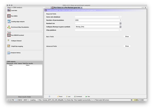
Place your cursor on a parameter name to see a brief description of the parameter.

Required Fields lists parameters that are essential for the analysis. Enter values for these parameters before starting the analysis.

• Gene sets database. Click the ellipse (…) button and select one or more gene sets:
  • GeneMatrix (from website) lists the MSigDB gene sets hosted on the GSEA-MSigDB file servers. These gene set files may contain hundreds of gene sets. See Exporting Gene Sets from MSigDB on how create gene set files containing only a subset of MSigDB gene sets of interest.
  • GeneMatrix (local gmx/gmt) lists the gene set files that you have loaded (see Loading Data).
  • GeneSets(grp) lists gene sets that GSEA has created in memory; for example, gene sets created using the Text Entry tab described below.
  • Subsets lists each gene set in each gmx/gmt file that you have loaded.
  • Text Entry allows you to create a gene set by entering the genes for that gene set; enter one gene per line. The gene set is deleted when you exit from GSEA.
• Number of permutations. Specify the number of gene_set permutations to perform in assessing the statistical significance of the enrichment score. It is best to start with a small number, such as 10. After the analysis completes successfully, run it again with a full set of permutations. The GSEA recommends 1000 gene_set permutations.
• Ranked list. Select a ranked list file (rnk) that you have loaded into GSEA.

If necessary, create a ranked gene list file (rnk) that defines the list of ranked genes. For a description of this file format, see GSEA file formats. You can create and edit the file using any text editor. If you use Excel, be sure to save the file as a tab-limited text file. Load the file into GSEA, as described in Loading Data.

• Chip platform(s). Click the ellipse (…) button and select one or more DNA chip (array) annotation files:

  • Chips (from website) lists the chip annotation files hosted on the GSEA-MSigDB file servers.
  • Chips (local .chip) lists the chip annotation files that you have loaded (see Loading Data).

  This parameter is mandatory or optional depending on the value of the Collapse dataset to gene symbols parameter.

• Collapse/Remap to gene symbols:

  • Select “Remap_Only” (default) to have GSEA map each identifier in the expression dataset to its respective gene symbol. This operation does not perform any mathematical collapse and requires each input identifier to map uniquely to an output gene symbol. When you select “Remap_Only”, you must specify a chip annotation file (Chip platform parameter) and gene sets (Gene sets database parameter) that identify genes by the same namespace.
  • Select “No_Collapse” to use your ranked list as is (with its native feature identifiers). When you select this option, the chip annotation file (Chip platform parameter) is optional and you must specify gene sets (Gene sets database parameter) that identify genes using the same feature (gene or probe) identifiers as those used in your ranked list.
  • Selecting “Collapse” is not recommended for GSEAPreranked (see Best Practices for Creating and Running Your Ranked List). With this setting GSEA will collapse each probe set in the expression dataset into a single vector for the gene, which gets identified by its HGNC gene symbol. When you select “Collapse”, you must specify a chip annotation file (Chip platform parameter) and gene sets (Gene sets database parameter) that identify genes by the same namespace.

  For more information, see Consistent Feature Identifiers Across Data Files.

Basic Fields lists additional parameters with standard defaults. Typically, you use the default values for these parameters. Click Show/Hide to display and hide these parameters.

• Analysis name. A short descriptive label for the analysis. The name cannot include spaces. This label is used as a prefix when naming the output report generated by the analysis (for example, my_analysis.CollapseDataset.1130510139575.rpt).

• Enrichment statistic. To calculate the enrichment score, GSEA first walks down the ranked list of genes increasing a running-sum statistic when a gene is in the gene set and decreasing it when it is not. The enrichment score is the maximum deviation from zero encountered during that walk. This parameter affects the running-sum statistic used for the analysis. The last section of the Gene Set Enrichment Analysis PNAS paper shows the mathematical descriptions of the methods used in GSEA. This option controls the value of p used in the enrichment score calculation shown there:

  • classic: p=0
  • weighted: (default). p=1
  • weighted_p2: p=2
  • weighted_p1.5: p=1.5

• Max size. After filtering from the gene sets any gene not in the expression dataset, gene sets larger than this are excluded from the analysis.

• Min size. After filtering from the gene sets any gene not in the expression dataset, gene sets smaller than this are excluded from the analysis.
• Save results in this folder. Path of the directory in which to place the analysis results. Existing results in this folder are not overwritten. By default, analysis results are saved in the GSEA output folder. To view this folder, select Help>Show GSEA output folder.

Advanced Fields lists parameters that control details of the GSEA algorithm and its Java implementation. Do not change the default values of these parameters unless you are conversant with the algorithm and its Java implementation. Click Show/Hide to display and hide these parameters.

• Collapsing mode for probe sets => 1 gene. Used only when the Collapse dataset to gene symbols parameter is set to True. Select the expression values to use for the single identifier that will represent all identifiers for the gene:

  • Max_probe (default): for each sample, use the maximum expression value for the identifiers. For example:

    Probeset_A	10	20	15	200
    Probeset_B	100	105	110	95
    gene_symbol_AB	100	105	110	200

  • Median_of_probes: for each sample, use the median expression value for the identifiers.

  • Mean_of_probes: for each sample, use the mean expression value for the identifiers.
  • Sum_of_probes: for each sample, sum the values of the identifiers.

• Normalization mode. Method used to normalize the enrichment scores across analyzed gene sets:

  • meandiv (default): GSEA normalizes the enrichment scores as described in Normalized Enrichment Score (NES).
  • none: GSEA does not normalize the enrichment scores.
• Omit features with no symbol match. Used only when Collapse/Remap to gene symbols is set to “Collapse” or “Remap_Only”. By default (true), the new dataset excludes probes/genes that have no gene symbols. Set to False to have the new dataset contain all probes/genes that were in the original dataset.
• Make detailed gene set report. Set to True (default) to create a detailed gene set report for each enriched gene set.
• Plot graphs for the top sets of each phenotype. Generates summary plots and detailed analysis results for the top x genes in each phenotype, where x is 20, by default. The top genes are those with the largest normalized enrichment scores.
• Seed for permutation. Seed used to generate a random number for phenotype and gene_set permutations: timestamp (default), 149, or user input. The specific seed value (149) generates consistent results, which is useful when testing software.
• Make a zipped file with all reports. Set to True (default=false) to create a zip file of the analysis results. The zip file is saved to the GSEA output folder with all of the other files generated by the analysis.

Buttons at the bottom of the page: - Help. Displays this documentation. - Reset. Restores the default values for all parameters. - Last. Loads the data used the last time you ran this analysis. - Command. Displays the command line used to run the analysis, as described in Running GSEA from the Command Line. - Run. Starts the analysis.

CollapseDataset Page#

CollapseDataset creates a new dataset by collapsing all probe set values for a gene into a single vector of values. The new dataset uses gene symbols as the gene identifier format. When you use the new dataset in a gene set enrichment analysis, be sure that your gene sets and array annotations also use gene symbols as the gene identifier format. For more information, see Consistent Feature Identifiers Across Data Files.

Note: By default, when you use the Run GSEA icon to run the gene set enrichment analysis, GSEA uses the CollapseDataset tool to collapse the dataset before running the gene set enrichment analysis. For more information, see the Collapse dataset to gene symbols parameter on the Run GSEA Page.

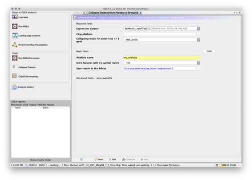
Place your cursor on a parameter name to see a brief description of the parameter.

Required Fields lists parameters that are essential for the analysis. Enter values for these parameters before starting the analysis.

• Expression dataset. Select your expression dataset from the drop-down list. If the dataset is not listed, you have not yet loaded it; see Loading Data.
• Chip platform(s). Click the ellipse (…) button and select one or more DNA chip (array) annotation files:
  • Chips (from website) lists the chip annotation files hosted on the GSEA-MSigDB file servers.
  • Chips (local .chip) lists the chip annotation files that you have loaded (see Loading Data).

• Collapsing mode for probe sets => 1 gene. Select the value to use for the single identifier that will represent all identifiers for the gene:

  • Max_probe (default): for each sample, use the maximum expression value for the identifiers. For example:

  Probeset_A	10	20	15	200
  Probeset_B	100	105	110	95
  gene_symbol_AB	100	105	110	200

  • Median_of_probes: for each sample, use the median expression value for the identifiers.
  • Mean_of_probes: for each sample, use the mean expression value for the identifiers.
  • Sum_of_probes: for each sample, sum the values of the identifiers.

Basic Fields lists additional parameters with standard defaults. Typically, you use the default values for these parameters. Click Show/Hide to display and hide these parameters.

• Analysis name. A short descriptive label for the analysis. The name cannot include spaces. This label is used as a prefix when naming the output report generated by the analysis (for example, my_analysis.CollapseDataset.1130510139575.rpt).
• Omit features with no symbol match. By default (true), the new dataset excludes features (genes) that have no gene symbols. Set to False to have the new dataset contain all features (genes) that were in the original dataset.
• Save results in this folder. Path of the directory in which to place the analysis results. Existing results in this folder are not overwritten. By default, analysis results are saved in the GSEA output folder. To view this folder, select Help>Show GSEA output folder.

Buttons at the bottom of the page:

• Help. Displays this documentation.
• Reset. Restores the default values for all parameters.
• Last. Loads the data used the last time you ran this analysis.
• Command. Displays the command line used to run the analysis, as described in Running GSEA from the Command Line.
• Run. Starts the analysis.

Preferences Window#

To display the Preferences window, select File>Preferences. Use this window to set GSEA configuration options.

General Settings#

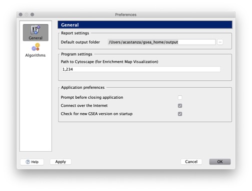
• Report settings:

  • Default output folder. When you run an analysis, by default, the results are written to this folder. To view this folder from GSEA, select Help>Show GSEA output folder.

  Note: If you choose a new folder, previously run reports remain in the old folder, unless you choose to move them.

• Program settings:

  • Path to Cytoscape (for Enrichment Map Visualization).
• Application preferences:
  • Prompt before closing application. When selected, if you close the GSEA application by clicking the X icon in the upper right corner, GSEA prompts you to confirm that you want to exit the application.
  • Connect over the internet. When selected, the Gene sets database and Chip platform(s) parameters (on pages such as the Run GSEA page) displays data files hosted on the GSEA-MSigDB file servers. If you are working offline, clear this option to disable this feature and avoid a time-consuming attempt to connect to the internet.
  • Check for new GSEA version on startup. When selected, on application startup GSEA will connect to the GSEA website to determine if a new application version is available and notify the user if an update exists.

Algorithm Settings#

• Use median instead of mean for metrics. Changes the default value of the Median for class metrics parameter on the Run GSEA page, which changes the Metrics for Ranking Genes. If you change this option, the new default value takes effect when you restart GSEA. By default, this option is not selected.
• Fix metrics for low variance. When calculating the ranking metrics, as described in Metrics for Ranking Genes, the denominator may be zero (0). A denominator of zero (0) causes an error in the analysis unless this option is selected. By default, this option is selected.
• Use biased variances. When calculating the ranking metrics, as described in Metrics for Ranking Genes, GSEA uses an unbiased variance to calculate standard deviation. Select this option to have GSEA use a biased variance instead.

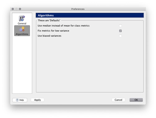
MSigDB XML Browser#

The MSigDB XML browser is a separate application available from the GSEA website downloads page. Use the MSigDB XML Browser to explore the gene sets and to export the gene sets of interest to gene set files that can be used with the gene set enrichment analysis.

To display the latest gene sets on the Browse MSigDB page, click the Load database button.

Note that you can also use this window to upload archived MSigDB files. For example, to load the MSigDB files from the v6.2 release, enter "msigdb_v6.2.xml" in the File path or URL to the MSigDB database field and click the Load database button.

You can upload multiple versions of MSigDB and toggle between them by clicking their respective tabs.

Use the filter field and the QuickFilterPane to filter the gene sets displayed in the table. GSEA displays gene sets that meet both the filter field AND quick filter criteria that you specify:

• The filter field is a text filter. As you enter text in the field, GSEA updates the list of gene sets to show only those that match that text. To change the text search options, click on the magnifying glass, as shown below:

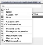
The filter shown above uses the default options All, Case insensitive, and Match anywhere to display all gene sets that have the characters “ca” anywhere in any column. To display gene sets whose names begin with the characters “ca”, click the NAME and Match from start options.

• The QuickFilterPane filters gene sets based on the values in four key columns. When you select a value for a column in the QuickFilterPane, GSEA updates the list of gene sets to show only those that have the selected value in that column. For example, to display only Human gene sets, select Human from the Species column in the QuickFilterPane.

The Deep Search Options provide more advanced search options:

• Find Sets that overlap with my set prompts you for a gene set and a name for the search results. All genes in the gene sets should be specified as HGNC gene symbols. You can select a gene set that you already created in memory or enter the genes for a gene set:
  • GeneSets(grp) lists gene sets that have created in memory; for example, gene sets created using the Text Entry tab described below.
  • Text Entry allows you to create a gene set by entering the genes for that gene set; enter one gene per line. The gene set is created in memory and deleted when you exit from GSEA.
• Find sets that contain this gene prompts you for a gene (case insensitive HGNC gene symbol) and a name for the search results. GSEA finds all gene sets that contain the specified gene. For example, you might search for VAMP2.

When you select a Deep Search Option, GSEA performs the search and displays the results in a new tab identified by the name you supplied. The original MSigDB page remains displayed in a separate tab, as shown below:

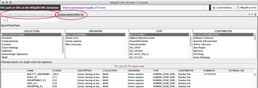
To export gene sets from the MSigDB to a gene set file that can be used with GSEA:

1. Select one or more of the gene sets in the table on the MSigDB page. To select multiple gene sets, use SHIFT-Click or CTRL-click.
2. Click Export sets as GeneSetMatrix. GSEA displays the following window:

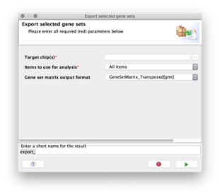
3. Select the target chip. Click the ellipse (…) button and select one or more DNA chip (array) annotation files:

   • Chips (from website) lists the chip annotation files hosted on the GSEA-MSigDB file servers.
   • Chips (local .chip) lists the chip annotation files that you have loaded (see Loading Data).

   GSEA uses Chip2Chip to translate the gene identifiers in the gene sets from HGNC gene symbols to the probe identifiers for the selected DNA chips.

4. Select the items to export:

   • All items: exports all gene sets displayed in the table on the MSigDB page.
   • Selected items: exports only the selected gene sets in the table on the MSigDB page.

5. Select the file format for the gene set file. Typically, you want to select gmt.

6. Enter a name for the resulting gene set file.
7. Click OK. GSEA writes the gene sets file to the default output folder (Help>Show GSEA output folder).

Appendix A: GSEA Error Codes#

Error 1001#

None of the gene sets that you specified passed the size threshold. Check that the selected gene sets:

1. Contain more than the minimum number of genes. The minimum gene set size is set by the Min size parameter (by default, 15).
2. Contain fewer than the maximum number of genes. The maximum gene set size is set by the Max size parameter (by default, 500).
3. Use the gene identifiers appropriate for this analysis:
   If you are collapsing your dataset (Collapse dataset to gene symbols parameter = True), the genes in the collapsed dataset are identified by gene symbol, so the gene identifiers in your gene sets must be gene symbols.
   If you are not collapsing your dataset (Collapse dataset to gene symbols parameter = False), the gene identifiers in your gene sets must be the same as those in your expression dataset.

For more information about "appropriate" gene identifiers, see Consistent Feature Identifiers Across Data Files.

Illumina data: The probe identifiers for Illumina chips contain leading zeros. Certain programs, such as Excel, automatically remove leading zeros. If you are collapsing your dataset, the probe identifiers in your dataset must match the probe identifiers in the chip annotation file. If this error occurs and you are using Illumina data, check that the probe identifiers in your dataset include the leading zeros.

Error 1002#

When you set the Collapse/Remap to gene symbols parameter to "Collapse" or "Remap_only", you must select one or more chip annotation files using the Chip platform(s) parameter.

Setting the Collapse/Remap to gene symbols parameter to "Collapse" tells GSEA to collapse each probe set in the dataset to a single vector for the gene, which gets identified by its HUGO gene symbol. In contrast, "Remap_only" uses the information in the chip to perform simple, non-mathematical translations of gene identifiers from one format to another. To do these operations, GSEA needs to map the probes in the dataset to their matching HUGO gene symbols. The chip annotation file(s) supply that mapping information. For more information, see DNA Chip (Array) Annotations.

Alternatively, you can set the Collapse/Remap to gene symbols parameter to "No_Collapse". In this case, GSEA does not perform any mapping operations on your dataset and the Chip platform(s) parameter is not used.

Error 1005#

GSEA attempted to collapse each probe set in the dataset to a gene, but there was no data in the resulting dataset. The most likely reasons for this are:

• You are attempting to collapse a dataset that is already collapsed.
• The probe identifiers in your dataset do not match the probe identifiers in the chip files selected in the chip platform(s) parameter.

Check the gene/probe identifiers in your dataset. If they are HUGO gene symbols, set the Collapse dataset to gene symbols parameter to False; the dataset is already collapsed. Otherwise, check that the probe identifiers in your dataset match the probe identifiers listed  in the chip file that you selected in the chip platform(s) parameter. For more information, see Consistent Feature Identifiers Across Data Files.

Error 1006#

The metric that you selected in the Metric for ranking genes parameter (Signal2Noise or tTest) requires that you have at least three samples for each phenotype. You have too few samples for at least one of the phenotypes selected in the Phenotype labels parameter.

To analyze a categorical phenotype that has fewer than three samples, use one of the following ranking metrics:

• Ratio_of_classes
• log2_Ratio_of_classes
• Diff_of_classes

For information about the metrics, see the Metric for ranking genes parameter on the Run GSEA Page.

For information about phenotypes, see Phenotype Labels.

Error 1010#

You selected a categorical phenotype for the Phenotype labels parameter; however, the metric that you selected in the Metric for ranking genes parameter is used with continuous phenotypes. Select one of the following metrics for a  categorical phenotype:

• Signal2Noise (default)
• tTest
• Ratio_of_Classes
• Diff_of_Classes
• log2_Ratio_of_Classes

For information about phenotypes, see Phenotype Labels.

For information about the metrics, see the Metric for ranking genes parameter on the Run GSEA Page.

Error 1011#

You selected a continuous phenotype for the Phenotype labels parameter; however, the metric that you selected in the Metric for ranking genes parameter is used with categorical phenotypes. Select one of the following metrics for a  continuous phenotype:

• Cosine
• Euclidean
• Manhattan
• Pearson

For information about phenotypes, see Phenotype Labels.

For information about the metrics, see the Metric for ranking genes parameter on the Run GSEA Page.

Error 1020#

Multiple identifiers mapped to a single gene in "Remap_Only" mode#

GSEA's "Remap_Only" collapsing mode is designed to convert gene identifiers across transcriptome versions, but does not perform any mathematical operations to handle multiple input symbols mapping to the same output symbol. The GSEA application only supports single instances of a given gene symbol in an analysis run. When GSEA encounters the case of multiple instances of the same gene symbol, the first instance is retained and the later instances are arbitrarily discarded. In order to prevent producing this arbitrary output, when multiple input values mapping to a single output value are encountered in Remap_Only mode, the attempt to remap symbols fails and returns Error 1020.

In order to remedy this error, it is recommended to choose an appropriate mathematical collapse function for the input data set, whereby multiple identifiers corresponding to the same gene will be collapsed to a single entry in the output file.

GSEA supports the following options for performing this mathematical collapse:

• Max_probe
• Median_of_probes
• Mean_of_probes
• Sum_of_probes

Appendix B: CHIP File Selection Help#

The 4.3.0 version of GSEA introduced support for the new gene set database files and chip files to support native analysis of mouse data first made available with MSigDB v2022.1.

These files are now split into two different tabs in both the GSEA gene sets and chip files UI windows.

Gene set files from the Human Collections have the suffix ".Hs.symbols.gmt" following the MSigDB version (v2022.1 in this initial release), gene set files from the Mouse Collections have the suffix ".Mm.symbols.gmt". Gene set files from the Human Collections have their contents provided in HGNC Gene Symbols, gene set files from the Mouse Collections have their contents provided in MGI Gene Symbols. These symbols follow different canonical formats (i.e. MTOR for human vs. Mtor for mouse).

As such, it is critical to pick CHIP files that map your data into the appropriate namespace (either human or mouse symbols).

Therefore, if a gene set file from the Human Collection (MSigDB) window is selected, you must also select a CHIP file from the Human Collection Chips (MSigDB) tab of the Chip platform selector window, and if a gene set file from the Mouse Collection (MSigDB) window is selected, you must also select a CHIP file from the Mouse Collection Chips (MSigDB) tab of the Chip platform selector window.

Chip files, like gene set database files are versioned and have a species specific suffix, i.e. ".Hs.chip" following the MSigDB version (v2022.1 in this initial release) for files targeting the Human Collections, and ".Mm.chip" for files targeting the Mouse Collections.

Both Human Collection Chips, and Mouse Collection Chips contain a full complement of Chips for native as well as orthology based analysis. Chips from the Human Collection Chips tab (files ending in .Hs.chip) that begin with Human_ convert human gene IDs to human symbols, files from this tab (still with the .Hs.chip suffix) that begin with Mouse_ or Rat_ will also have the text "Human_Orthologs" in the file name, and when used will apply orthology mapping data to convert the dataset to match the human gene symbols namespace of the MSigDB Human Collections database.

Likewise, chips from the Mouse Collection Chips tab (files ending in .Mm.chip) that begin with Mouse convert mouse gene IDs to mouse symbols, files from this tab (still with the .Mm.chip suffix) that begin with Human or Rat_ will also have the text "Mouse_Orthologs" in the file name, and when used will apply orthology mapping data to convert the dataset to match the mouse gene symbols namespace of the MSigDB mouse Collections database.

So, if the gene set database file c5.go.bp.v2022.1.Hs.symbols.gmt was selected from the Human Collection's tab, the appropriate CHIP file regardless of dataset species would be one of the _MSigDB.v.2022.1.Hs.chip files available from the Human Collection CHIPs (MSigDB) tab, and if the gene set database file m5.go.bp.v2022.1.Mm.symbols.gmt was selected from the Mouse Collection's tab the appropriate CHIP file regardless of dataset species would be one of the _MSigDB.v.2022.1.Mm.chip files available from the Mouse Collection CHIPs (MSigDB) tab.